Trading System #1–SPY VIX (Part 2)
Posted by Mark on October 1, 2012 at 06:04 | Last modified: September 21, 2012 06:58In http://www.optionfanatic.com/2012/09/28/trading-system-1-spy-vix-part-1/ (9/28/12), I introduced the concept of evolutionary operation and began to talk about the different variables present in this trading system. Today I want to continue that discussion from the perspective of optimization.
Investopedia.com defines optimization as:
“…the process of adjusting one’s trading system in an attempt to make it more effective. These adjustments include changing the number of periods used in moving averages, changing the number of indicators used, or simply taking away what doesn’t work.”
In the system development process, optimization is going to allow me to look at performance metrics for every combination of specified parameter values. In the present context, I will allow x to vary from 3-7 in increments of one [e.g. 3 (days), 4, 5, 6, or 7]. I will allow y to vary from 5-25 in increments of five [e.g. 5 (percent), 10, 15, 20, or 25]. I will allow z to vary from 6-15 in increments of one. The result of this process will be summary statistics for 5 * 5 * 10 = 250 trading systems.
The goal of optimization is not to find out which set of parameter values performed the best in order to trade those going forward. This is called “curve-fitting” and the reason optimization has gotten a bad name in some circles. The more variables you have and the greater the number of total parameter value combinations, the more unlikely you are to see similar performance in the future as seen in the most profitable backtest.
Rather, the goal of optimization should be to assess the performance landscape from one combination of parameter values to the next. Going back again to http://www.optionfanatic.com/2012/09/28/trading-system-1-spy-vix-part-1/ (9/28/12), I want to know if these performance graphs have spike regions or plateau regions. If they have spikes then I will discard them, considering performance to be lucky rather than good. If they have plateau regions then I want to choose parameter values near the middle of those plateaus (margin of safety).
In my next post I’ll start running the numbers.
Categories: System Development | Comments (2) | PermalinkTrading System #1–SPY VIX (Part 1)
Posted by Mark on September 28, 2012 at 05:31 | Last modified: October 1, 2012 05:35With the “motion to dismiss” now denied, the next step is to lay the groundwork for developing this strategy into a trading system.
As a review, the trading strategy is based on two claims. First, five days after the CBOE Volatility Index (VIX) closes 5% or more below its 10-day simple moving average (SMA), the S&P 500 index (SPX) has lost money on average. Second, when the VIX closes 5% or more above its 10-SMA, SPX has outperformed the average week better than 2-1 over the next five trading days.
The current system in development offers three variables to be backtested: x-bar stop y% extended from its z-SMA. In this case, we have used x=5 (five-day trades), y=5, and z=10 (VIX closing 5% above/below its 10-SMA). What we want to see in backtesting is solid results with these values. We also want to see solid results when we slightly change these values, though.
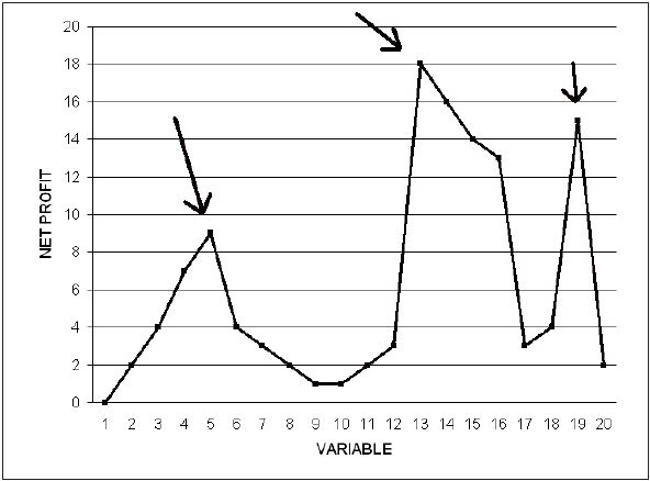
The process of “evolutionary operation” looks to keep one variable constant while changing another to see its effect on system performance. Graphically speaking, we want to plot some measure of performance (e.g. net profit) vs. the one variable being changed:
This does not have the appearance of a robust system because slight changes in the variable drastically affect net profit. Whether a moving average is four periods vs. five or 14 periods vs. 15 should not matter. If one value appears magically improved in the midst of mediocre results then those backtested profits are likely a matter of luck rather than the system taking advantage of consistent opportunity (and subsequent future profits).
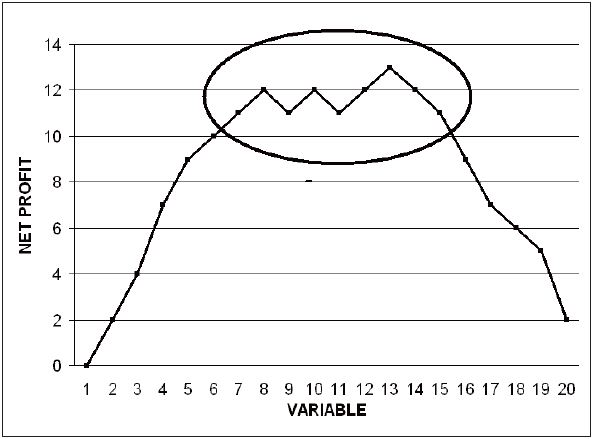
This is what we hope to see. All values from 6-15 produced solid profit for this trading system. Rather than the spikes in the previous graph we see a plateau region in this one. This should be a necessary (but not sufficient) condition for a system we might trade in the future with real capital.
These graphs were adapted from Tomasini and Jaekle (2009).
In my next post I will continue this discussion in terms of optimization.
Categories: System Development | Comments (2) | Permalink
Trading System #1–Brief Notes on Statistical Interpretation
Posted by Mark on September 18, 2012 at 07:24 | Last modified: September 19, 2012 06:14In addition to generating profit and loss numbers, sophisticated backtesting software will provide a whole slew of statistics each designed to address a different aspect of the performance results.
Without question, one of the most complicated matters in developing a system is how best to evaluate it. Different aspects will be more or less important to different people. One person may not care about the average win vs. average loss as long as most trades win. Another person may not care about how few trades win and how large the drawdowns get as long as net return is maximized over time. Younger people can afford to lose more because time is on their side. Retirees may be risk-averse because what they lose they don’t have so much opportunity to regain.
From a graphical point of view, many backtesting statistics describe the equity curve itself. Supposing a given initial value ($1M in our case), the equity curve shows the value of the account over time. A curve sloping up (down) is making (losing) money. Drawdowns are the difference (in dollars or percent) from an equity value peak to valley. Flat times describe time intervals between new equity highs. Most people prefer shallow drawdowns and shorter flat times to sleep easier at night. In theory, this may be achieved at the expense of total profit and exponential (sloping up more and more over time) equity curves. A lower total profit often means a safer system, however, that has a lower Risk of Ruin: probability of the account going to zero (“bust”) from a string of losses or just a couple large losses.
Like trading itself, much of system development is about tradeoffs.
Categories: System Development | Comments (0) | PermalinkStrategies vs. Systems (Part VI)
Posted by Mark on July 1, 2012 at 10:26 | Last modified: July 1, 2012 10:26In Part V of this series (http://www.optionfanatic.com/2012/06/05/strategies-vs-systems-part-v/), I concluded some commentary on discretionary trading. Today I want to provide some argument for algorithmic (also known as “rules-based” or “systematic”) trading.
Rules-based trading systems may be tested for statistical reliability. Robust systems have proven themselves over extended periods of time and different market environments. This leaves us confident about trading them into an unknown future.
Systematic trading eliminates decision making. An oft-cited quote is “prepare for war in a time of peace.” In the heat of battle, adrenaline kicks in. Decisions are then motivated by survival rather than profit. These are the times when psychic pain causes us to realize huge losses if only to sleep restfully at night. This is not the road to consistent profits over time.
Systematic trading ensures consistent application of trading rules. Rules without enforcement are trades without rules. No longer are we then trading systematically and no longer does our historical backtesting apply. Based on nothing concrete we are now gambling, not trading.
Systematic trading eliminates emotion. We program entries and exits to ensure they occur reliably and according to plan. One of the largest uncertainties of discretionary trading is our emotional reactions to pleasant or unpleasant situations. Systematic trading removes this.
Finally, systematic trading provides continuous risk control. Profit targets and stop-losses were determined through the rigorous system development process yielding potential results with which we feel comfortable. Gone will be the days of “I’ll hold on just a little longer because I think this market is about to reverse.” The trading platform will exit our trades automatically.
In my next post, I will address some potential downside to systematic trading.
Tags: critical thinking | Categories: System Development | Comments (1) | PermalinkOn Quantitative Trading
Posted by Mark on May 17, 2012 at 06:35 | Last modified: May 17, 2012 06:35“After the recent major losses at quantitative hedge funds, many people have started to wonder if quantitative trading is viable in the long term. Though the talk of the demise of quantitative strategies appears to be premature at this point, it is still an important question from the perspective of an independent trader. Once you have automated everything and your equity is growing exponentially, can you just sit back, relax, and enjoy your wealth? Unfortunately, experience tells us that strategies do lose their potency over time as more traders catch on to them. It takes ongoing research to supply you with new strategies.
There are always upheavals and major regime changes that may occur once every decade but will nevertheless cause sudden deaths to certain strategies. As with any commercial endeavor, a period of rapid growth will inevitably be followed by the steady if unspectacular returns of a mature business. As long as financial markets demand instant liquidity, however, there will always be a profitable niche for quantitative trading.”
–From Quantitative Trading (2009) by Ernest Chan
Categories: System Development, Wisdom | Comments (0) | PermalinkIntroduction to Profit Factor
Posted by Mark on April 24, 2012 at 10:51 | Last modified: April 24, 2012 10:52The profit factor (PF) is one of the most important statistics to calculate when developing a trading system.
PF is defined as total profits divided by total losses. Another way of stating this is:
average net profit on winning trades # winning trades
——————————————————- * ————————– (1.1)
average net loss on losing trades # losing trades
Although very similar, I would point out that PF is not exactly the same as a trading system’s expectancy (E):
Expectancy (E) = (Probability of Win * Average Profit) – (Probability of Loss * Average Loss)
E may be interpreted as the average gain or loss per dollar risked on a trade. PF may be interpreted as the number of dollars made per dollar lost. A successful trading system should have E > 0 and PF > 1.
Maintaining a relative equivalence between average losses and average gains is one way to run a successful income trading business. Consider a trading strategy that sells 20 naked puts per month for $2.00 each to collect $4,000. These puts are so far out of the money that only a very rare event will result in a loss. Eventually, October 2008 happens and this very consistent trade suddenly loses $396,000. Not only did this one month just wipe out profits from your last 99, but the psychological devastation will likely result in a swift career change.
The PF calculation gives us the minimal requirements by which to profit through income trading. If a strategy’s average losses are three times its average gains then the second term of (1.1) must equal at least 3 for PF to exceed 1. That is, three trades must win per every trade lost: a win rate of 75%. Similarly, if the strategy loses twice as much as it usually gains then it must win 67% of the time to break even.
I will build on this concept of PF in my next post with an introduction to Sizing Risk.
Tags: trader education | Categories: System Development | Comments (1) | PermalinkTo Optimize or Not to Optimize?
Posted by Mark on March 15, 2012 at 11:44 | Last modified: March 15, 2012 11:54In the quest for consistent trading profits, backtesting is generally regarded as useful but optimization is viewed by some as a four-letter word.
If a system captures profits from consistent human behavioral characteristics reflected in the market then the past should reasonably approximate the future. This will never be perfect but it may be profitable.
Optimization is the determination of what trading parameters applied to past market action would have resulted in maximal returns. After all, if it worked well in the past then shouldn’t be likely to work in the future if the past is at least some small reflection of the future due to those consistent behavioral characteristics? This is called curve-fitting.
One of the biggest scams on Wall Street is to present a system with brilliant historical returns (anyone can run an optimization procedure on backtested data to do this) and sell it as a system to be used in live trading. Trading an optimized system into the future is almost guaranteed to underperform the past. Selling an optimized system can be like selling snake oil, and charlatans abound in financial circles who aim to do just that.
To avoid excessive curve-fitting, some think that if you don’t optimize then you can’t fall prey to the illusion. Choose only one parameter value and backtest it; if you come up with impressive results then they’re likely to persist into the future, right?
Not necessarily!
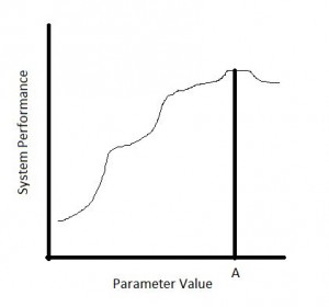
Suppose a system has one parameter (e.g. period for a moving average). Imagine backtesting the system repeatedly over the historical time period while changing the period each time. When you plot performance, does it look like this…
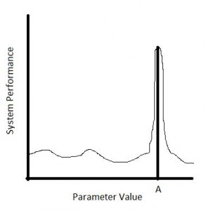
…or like this?
In both cases, using a period of A would have resulted in the best historical performance. However, in the latter case, if the period varied just a tad higher or lower then system performance was devastated. In the former case, trading with a period higher or lower than A would still have generated solid performance. Since the past is never identical to the future, which do you think has a better chance of generating profits going forward?
The bottom line is that “curve-fitting” and “optimization” are not four-letter words if used to know what you do not know. Optimize not with the intent of finding the perfect parameter to trade going forward. Optimize with the intent to determine whether encouraging past results are likely to persist into the future.
Tags: critical thinking, survival, trader education | Categories: System Development | Comments (0) | Permalink


