Portfolio Margin Considerations with the Automated Backtester (Part 1)
Posted by Mark on December 6, 2018 at 06:40 | Last modified: October 24, 2018 11:51I want to revisit something mentioned in Part 1 about portfolio margin (PM).
Allocation and margin are two separate things with regard to short premium trades and I have only been taking into account the former. I have mentioned allocation with regard to serial backtesting of [non-overlapping] trades. After further consideration, I think margin should be monitored because while we may be able to place a trade, whether we can maintain the position when the market goes sharply against us is a different story.
At some brokerages, accounts of sufficient size can qualify for portfolio (also termed “risk-based”) margin (PM). Reg T margin [which applies to cash, not margin, accounts] reduces buying power by the maximum potential loss at expiration for a given trade. PM uses an algorithm that analyzes profit and loss of the whole portfolio when stressed X% up and Y% down. In other words, if the underlying security were to increase (decrease) by X% (Y%) today (not at expiration), then the algorithm calculates the worst change in value across that range. Specifics vary by brokerage but as an example, the algorithm may calculate -12% and +12% by increments of 3%. The maximum loss at any increment is the portfolio margin requirement (PMR). I will not incur a margin call provided PMR is less than the net liquidation value of my account.
Calculating PMR requires modeling of the cumulative position. A permanent component of the option pricing equation is implied volatility (IV). IV may be understood as the relative supply/demand for an option. This is inherently unknown, which is why a model is necessary.
As an example to explain this price uncertainty, suppose I am an institutional option trader looking to allocate $50 billion to a specific short premium position. The sooner I get this done, the sooner I have the opportunity to start making daily profit. Once the funds clear, I want to be in regardless of whether the market is up, down, a little or a lot.* You can be sure my $50 billion is going to move some markets by making purchased (sold) options more (less) expensive along with a coincident IV increase (decrease). This is the principle of supply and demand that, in this case, has nothing to do with underlying market move: simply when the bank/brokerage clears my funds for trading. For this and countless other reasons having nothing to do with market movement, unpredictable purchases/sales regularly occur—perhaps in smaller dollar amounts but the aggregate effects can be imagined to be similar.
I will continue next time.
* I may avoid “a lot” if liquidity dries up or bid/ask spreads become large.
Automated Backtester Research Plan (Part 5)
Posted by Mark on December 3, 2018 at 06:06 | Last modified: November 9, 2018 13:30Today I will finish up the automated backtester research plan for naked calls.
Once done studying daily [overlapping] trade statistics, we can repeat the naked put analysis with a serial trading strategy for naked calls. This involves one open trade at a time. We can look at number of trades, winning percentage, compound annualized growth rate (CAGR), maximum drawdown, risk-adjusted return, and profit factor. Again, equity curves will represent just one potential sequence of trades and some consideration can be given to Monte Carlo simulation. We can plot equity curves for different account allocations such as 10% to 70% of initial account value by increments of 10%.
With both overlapping (daily) and non-overlapping (serial) trades, position size should be held constant to allow for an apples-to-apples comparison of drawdowns throughout the backtesting interval. With naked puts, position size is notional risk. Naked calls, though, have unlimited notional risk. Maybe we deduct 0.05-0.20 for the naked call premium under the assumption that we always purchase the lowest strike call available for minimal price to limit margin.
This would result in a vertical spread, though, and the width would be different depending on underlying price.
Does this compromise the feasibility of naked call backtesting altogether? If calls must be done as vertical spreads then buying the long leg for minimal premium will be different from most call credit spread studies to be done for widths 10 (25) to 50 (100) points wide by increments of 10 (25)—except for very low underlying prices where the larger widths may result in the same minimally-priced long being purchased. The naked call study has then become a call credit spread study, which overlaps with the vertical spread backtesting to be detailed later. This deserves further deliberation.
We can apply the same rolling ideas to naked calls as we did to naked puts. We can roll naked calls [up and] out to the next month when a short strike is tested or when the trade is down 2-5x initial credit. We can also roll naked puts up to same original delta in the same or next month if strike gets tested.
When studying filters, it will be important to look at total number (and distribution) of trades along with equity curve slopes to determine consistency of profit. Risk-adjusted return and profit factor should also be monitored.
Naked call filters for study are similar to those for naked puts. We can look at trades taken at 5-20-day highs (lows) by increments of five. Trades can be taken only when a short-term MA is above (below) a longer-term MA. As mentioned in the Part 2 footnote, my preference would be to avoid getting overly concerned with period optimization, but this may be unavoidable. Implied volatility (IV) filters may include trades taken with IV at an X-day high (low), on the first down day for IV after being up for two consecutive days, or with IVR above 25/50.
I am curious to find out if naked calls can add to total return and/or lower standard deviation of returns.
Next time I will revisit margin considerations.
Categories: Backtesting | Comments (0) | PermalinkAutomated Backtester Research Plan (Part 4)
Posted by Mark on November 30, 2018 at 07:02 | Last modified: October 17, 2018 09:31Today I continue with the research plan for naked calls.
As discussed with puts, I think naked call trades should be normalized for notional risk.
I would like to see a distribution of naked call losers in time and in magnitude. Date can be on the x-axis with underlying closing price (line graph) on the right y-axis and trade PnL (histogram) on the left y-axis. It certainly makes sense to do these graphs for expiration. We can also do these graphs for managing winners at 50% (and/or 25%?) and for managing losers.
I suggested managing trades early (i.e. exiting at 7-21 DTE by increments of seven or exiting at 20-80% initial DTE by increments of 15%) for naked puts, but I did not mention it for calls. This is because in backtesting naked calls down to 7 DTE, I am not sure what kind of time stop makes sense. Four, three, and two DTE correspond to expiration Monday, Tuesday, and Wednesday respectively—any of which would seem to be an extremely short time to hold these trades. They could be repeated every week, though. This is subject for debate.
When the market rips higher, naked calls can lose quickly because they are closer to the money. This almost makes me more reluctant to trade naked calls than puts, which is counterintuitive because traditional wisdom says naked puts are most at risk. Naked puts are vulnerable to directional moves—equity markets tend to crash down farther (and faster) than they crash up—and extremely vulnerable to volatility explosion. If volatility affects naked calls at all on strong upside moves then it generally benefits them (going from inflated IV on a pullback to normal/low IV after the rebound). The culprit hiding in the shadows is vertical skew, which makes OTM calls cheap compared to OTM puts.
This line of discussion makes me curious to know how time stops can reduce risk of naked calls despite the above discussion of why they were not mentioned in the previous post. I would be interested in seeing a histogram of PnL (y-axis) by DTE (DIT): high (low) to low (high) moving from left to right along the x-axis. This plot would be for unmanaged trades. I would expect to find that earlier exits mitigate the most extreme losses—but at what cost?
The vertical skew discussion also implies that [if implemented then] naked calls should be traded in a smaller position size than naked puts. I would like the backtest to provide some insight about reasonable position sizing. I want to study the rolling (out or up and out) adjustment and how many rolls have been historically required during the sharpest and most sustained upside moves. As an example of how this could be relevant, suppose risk management is to roll into double the position size when premium increases by 100%. If we don’t think this will happen for more than three consecutive months, then maybe position size for naked calls should be 13% (or less) that of naked puts.
I will continue next time.
Categories: Backtesting | Comments (0) | PermalinkAutomated Backtester Research Plan (Part 3)
Posted by Mark on November 27, 2018 at 06:43 | Last modified: November 9, 2018 13:26Finishing up the discussion on filters, some can probably be tested on the underlying alone without the automated backtester. By looking just at underlying price we can plot trade distribution (looking for consistent vs. lumpy). Maximum adverse excursion can also be studied to see whether this improves with filter application. This type of analysis may lend itself more to spreadsheet work and macros. I have numerous research questions that would fit in this category.
Back to the automated backtester, I would like to study rolling as a trade management tool. We can roll naked puts [down and] out to the next month when a short strike is tested or when the trade is down 2-5x initial credit. We can also roll naked puts down to same original delta in the same or next month if strike gets tested.
Some thought may need to be given to calculate days in trade (DIT) for rolling adjustments. If rolling out doubles DIT, for example, then annualized ROI is halved. This may not be the best result. If I’m not looking to calculate [annualized] ROI then this may be a moot point, but we should be aware that for breakeven or normal profit, rolling will significantly increase DIT.
As an overlay, another adjustment I am interested in testing is the addition of an ATM short call to manage NPD.
Parts 1 and 2 of this research plan primarily addressed naked puts. The plan is similar for naked calls.
The first phase of naked call backtesting involves overlapping trades. We can study trades entered every day between 7-42 DTE. We can choose the first strike under 0.10 to 0.50 delta by increments of 0.10. We can hold to expiration or manage winners at 25% (ATM options only?) or 50%. We can manage losers at 2x, 3x, 4x, and 5x initial credit. I’d like to track and plot maximum adverse (favorable) excursion (no management) for the winners (losers) along with final PnL and total number of trades. I want to monitor winning percentage, average win, average loss, largest loss, profit factor, average trade (PnL), PnL per day, standard deviation of winning trades, standard deviation of losing trades, average DIT, average DIT for winning trades, and average DIT for losing trades.
My gut leans away from studying longer-term naked calls because of vertical index skew. With the market generally drifting higher and naked calls being cheaper than put counterparts (thereby implying NTM call sales for equivalent premium to farther OTM puts), my bias is toward shorter-term holdings. On the other hand, a 30-64 DTE backtest would allow for an apples-to-apples naked put comparison. This is subject for debate.
I will continue next time.
Categories: Backtesting | Comments (0) | PermalinkAutomated Backtester Research Plan (Part 2)
Posted by Mark on November 22, 2018 at 07:22 | Last modified: November 9, 2018 13:32Last time I discussed backtesting naked puts by opening one trade every day.
A final piece to managing winners is total number of trades. In a serial scenario, total trades would be greater for managing winners than holding to expiration whereas in a daily/overlapping trade scenario, total trades would be equal despite average daily notional risk being less for managing winners. It might make sense to track daily notional risk as a proxy for actual buying power reduction, which would be significantly less in a [portfolio] margin account and perhaps too complex (or not worth the effort) to build into the automated backtester.
The research plan continues with backtesting naked puts in a serial manner by having only one trade open at a time.
For the serial approach, I would like to tabulate several different statistics. These include total number of trades, winning percentage, compound annualized growth rate (CAGR), maximum drawdown, risk-adjusted return (RAR), and profit factor (PF). Equity curves will represent just one potential sequence of trades and some consideration could be given to Monte Carlo simulation. We can plot equity curves for different account allocations such as 10% to 70% of initial account value by increments of 5% or 10% for a $50M account. A 30% allocation (for example) would then be $15M per trade. Trade size should be held constant throughout in order to maintain apples-to-apples comparison of drawdowns throughout the backtesting interval.
The general principle behind filters is to achieve more profit (PnL per trade—sometimes as a result of decreasing drawdown or, in this case, a higher winning percentage) despite fewer trades. My preference is not to see a lumpy equity curve where a vast majority of trades occur on a small percentage of days. This gets away from trading as a business to pay the monthly living expenses. When studying filters, it will therefore be important to look at number of trades and the slope of the equity curves under different filters to determine consistency of profit. RAR and PF will also be useful.
Examples of filters to be tested are numerous. We can look at trades taken at 5-20-day highs (lows) by increments of five. Trades can be taken only when a short-term MA is above (below) a longer-term MA.* Trades can be avoided when the underlying is under the 20-, 50-, or 200-day MA. IV at an X-day high may be a useful inclusion or exclusion filter (always minding sufficient sample size at extreme parameter values). Trade entry can be filtered by IV rank (perhaps 25% or 50% with a period of 30, 180, or 365 days). A volatility stop could be implemented to exit losing trades if IV increases by 30-100% using increments of 10%.
I will continue next time.
* Some thought would have to be given to period determination. I do not want to get into an extensive optimization game
since I’m more a believer in Occam’s Razor (i.e. K.I.S.S.).
Automated Backtester Research Plan (Part 1)
Posted by Mark on November 19, 2018 at 05:46 | Last modified: October 17, 2018 07:54Today I begin outlining a research plan for the automated backtester.
I want to start with naked puts because they employ the least leverage.
We can study trades entered every day between 30-64 DTE. We can choose the first strike under -0.10 to -0.50 delta by increments of -0.10. We can hold to expiration, manage winners at 25% (ATM options only?) or 50%, or exit at 7-21 DTE by increments of seven. We can also exit at 20-80% of the original DTE by increments of 15%. We can manage losers at 2x, 3x, 4x, and 5x initial credit. I’d like to track and plot maximum adverse (favorable) excursion (no management) for the winners (losers) along with final PnL and total number of trades. I want to monitor winning percentage, average win, average loss, largest loss, profit factor, average trade (average PnL), PnL per day, standard deviation of winning trades, standard deviation of losing trades, average days in trade (DIT), average DIT for winning trades, and average DIT for losing trades.
Return on investment (ROI) does not seem relevant for naked puts because of the large notional risk. At the moment, I cannot think of a need to track buying power reduction, but this is something I will keep in mind.
Speaking of notional risk, unless normalized the average win/loss can vary significantly based on underlying price (and option prices). We can apply a fixed position size (e.g. $5M) and calculate number of contracts for each trade. If I am selling a 1500 put, for example, then $5M divided by $150,000 (notional risk) is 33 contracts ($4,950,000) and change (truncate). If I sell a 1000 put then 50 contracts would amount to $5M notional risk. Regardless of underlying price, this will give a variable number of contracts to keep notional risk relatively constant thereby keeping profits and losses commensurate.
If we don’t normalize for notional risk then we would get numbers that don’t make as much sense. With the underlying at 1000 vs. 2000, for example, the contribution to the total PnL would be roughly twice as large at the higher prices. The overall contribution should not significantly vary based on an arbitrary factor.
I want to briefly discuss the relative constancy around target position size. I mentioned that $4,950,000 is 1% less than $5,000,000. As discussed here, I would expect this error to be inversely proportional to number of contracts because the percentage difference between consecutively decreasing integers increases (e.g. 19 is 5% lower than 20 whereas 9 is 10% lower than 10). If we deem this error to be too large—especially for lower-priced underlyings like RUT—then the target position size can be increased (e.g. from $5M to $10M).
I would like to see a distribution of losers in time and in magnitude. Date can be on the x-axis with underlying closing price (line graph) on the right y-axis and trade PnL (histogram) on the left y-axis. It certainly makes sense to do these graphs for expiration. We can also do the graphs for managing winners at 50%. I think it also makes sense to do these graphs for managing early (e.g. 7-21 DTE or X% of the original DTE) as well as managing losers.
I will continue next time.
Categories: Backtesting | Comments (0) | PermalinkPut Credit Spread Study 1 (Part 4)
Posted by Mark on October 30, 2017 at 07:38 | Last modified: August 14, 2017 13:58Today I will present data obtained from the methodology discussed here.
I started by adding $40 to each trade to represent the lower transaction fee. Going from $0.26/contract to $0.16 represents $10 per leg and the trade has two legs each to open and to close: 4 * $10 = $40.
I then recalculated and identified trades with ROI smaller than the -25% SL. I found 188 trades.
I then identified the original SL dates and looked at the chart to determine if these were bottoms. If so then I was probably looking at a flip. If not then I still had a loser and I would have to retest to see how big the loser would be.
This is when I realized that regardless of proposed alternatives, I would have to retest the 188 trades anyway. The previous step identified 40 trades as flip candidates. While that seemed encouraging, I only had part of the picture.
I proceeded to replace the original values of Exp ROI w/25% SL with 188 retested values. I then recalculated trade statistics.
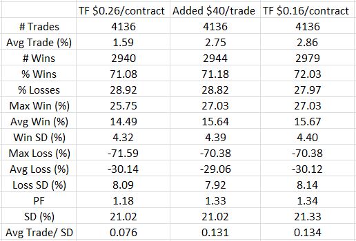
Here are the results:
The third column is an approximation. While accounting for the lesser TF, it neither takes into account flips nor new PnL values for trades evading SL the original day only to trigger SL on a subsequent day.
To see the impact of lowering TF, therefore, the second and fourth columns should be compared. Doing so reveals an improvement in most of the statistics. I don’t see any surprises here. Simply adding $40 per trade is $40 / ($4000 – $40) = 1.01% on net margin. The average trade improved by 1.27%, which seems reasonable when flips are taken into account. Average loss remained about the same and 39 fewer trades actually lost with the lowered TF.
I think the moral of the story is that once again, execution makes a big difference. I am tempted to repeat the process for TF $0.06 but I think there may be cases where options priced $5.00 to $15.00 may incur more than nickel slippage. $0.16/contract may therefore be painting a realistic picture.
Another repetitive theme is the temptation to take only those trades that have gone against me by the slippage amount to improve the effective price. Profitable trades from inception throughout would go unable. Would this missed opportunity more than offset the benefit of improved entry price on all the others? That is the critical question.
Categories: Backtesting | Comments (0) | PermalinkBacktesting Frustration (Part 8)
Posted by Mark on October 6, 2017 at 07:04 | Last modified: August 7, 2017 10:31Recall that my impetus for resurrecting this “Backtesting Frustration” blog series was the realization that I cannot use quick spreadsheet manipulations and calculations to reprocess 188 backtrades with lower transaction fees (TF). Today I want to go through a sampling of chart action showing different cases of false and real bottoms.
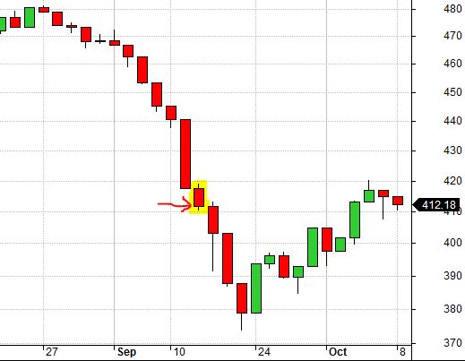
The highlighted candle below is a false bottom from 9/18/2001:
The SL would be triggered in subsequent days even if it was not triggered here due to lower TF.
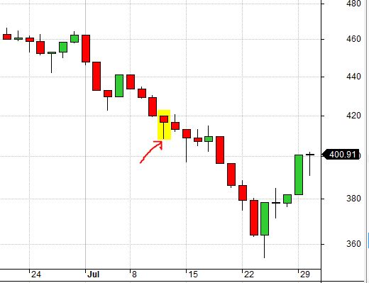
The highlighted candle below is a false bottom from 7/11/2002:
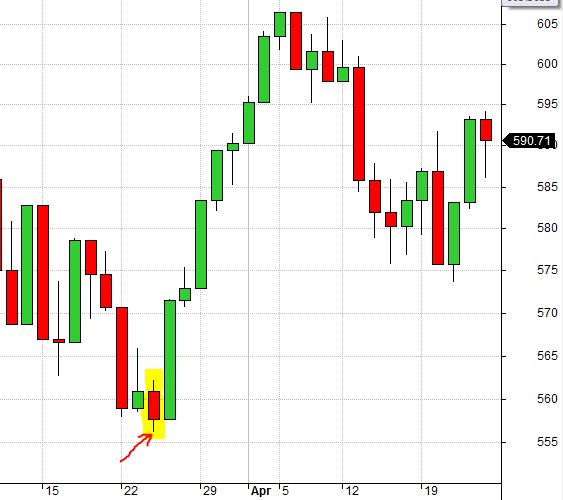
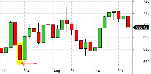
The highlighted candle below is a real bottom from 3/24/2004:
Because SL was not triggered two days earlier, this was the last downside move capable of taking the trade out at a loss. Smaller TF (slippage) would allow the position to evade SL and proceed to full profit.
Here is another real bottom from 7/21/2006:
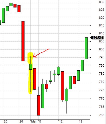
This is a false bottom from 3/1/2007:
Because I backtest [once] daily, long wicks (as shown here) represent price extremes that may or may not force trade exit depending on what time intraday (see 5/6/2010 candle, below) they occur.
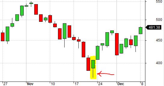
Here is a real bottom from 11/21/2008:
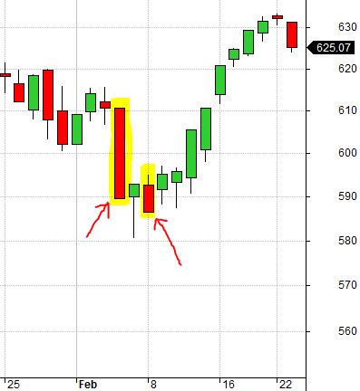
These are real bottoms from 2/4/2010 and 2/8/2010:
While the market went a few points lower on 2/8/2010, being close to February expiration allowed accelerated time decay to offset the move. Were this a March position, 2/4/2010 probably would have been a false bottom.
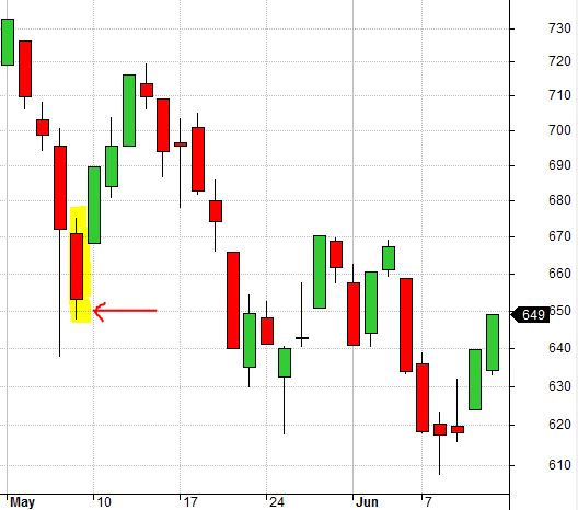
Here is a false bottom from 5/7/2010:
This would have been a real bottom for a May position but with the additional month to expiration, the market had time to recover and then fall once again.
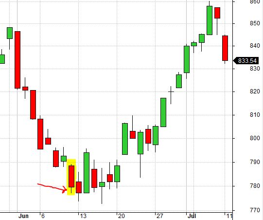
Here is a false bottom from 6/10/2011:
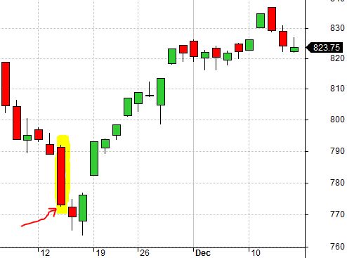
Here is a false bottom from 11/14/2012:
Real bottom from 8/30/2013:
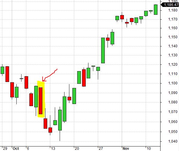
False bottom from 10/9/2014:
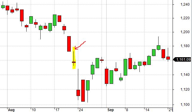
False bottom from 8/21/2015:
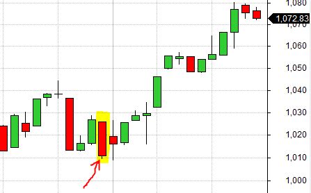
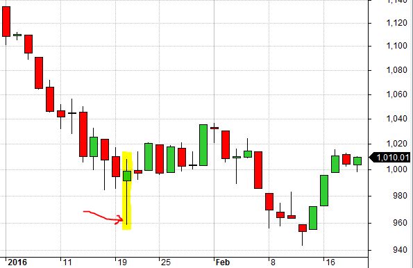
Here is a false bottom from 1/20/2016:
This is another big wick but a lot can happen with several weeks to expiration.
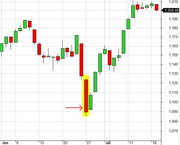
Finally, here is a real bottom from 6/27/2016:
While spreadsheets are great at managing large volumes of data and allowing us to do computational operations quite efficiently, we also have to be cognizant of what information they do not reveal. Besides outright fraud, I believe oversights like these are a major contributor to falsely optimistic backtesting results. This is a good reason why even advanced traders are best advised to undertake system development with others capable of proofreading the work.
Categories: Backtesting | Comments (0) | PermalinkBacktesting Frustration (Part 7)
Posted by Mark on October 3, 2017 at 06:35 | Last modified: August 2, 2017 13:18Today I resume my series on backtesting frustrations by talking about the frustration of “flips.”
I mentioned this in Part 1 with regard to recalculating results with different TF values. A trade that is down 25.5% with $0.26/contract may only be down 24.5% at TF $0.16/contract thereby evading the trigger of SL and ending up profitable. Simply recalculating the results, I thought, would overlook these flips (from loser to winner) altogether.
In taking a closer look at the put credit spread results I see that 188 out of 1,093 trades originally hitting the -25% SL show a loss smaller than -25% with $40/trade added.
I can now proceed in a few different ways: 1. Redo the 188 trades with TF $0.16 ($0.06)/contract; 2. Assume the SL was not hit and use either 7 DTE or Exp PnL values instead; 3. Assume these 188 trades closed for zero gain/loss.
Without doubt, the first option would be most accurate and also the most time-consuming.
I therefore started working with option #2 until I realized a major problem with the assumption. A trade that evades SL on one day may still hit SL on a subsequent day. Being so close to SL, another down day would probably trigger the unprofitable exit. With the market showing recent bearishness this seems quite feasible.
Furthermore, if the subsequent down day is big then the loss might end up being much greater than initially recorded.
Option #3 was intended to be a more conservative form of #2. In [falsely] thinking most of these trades avoiding SL would flip, it occurred to me that the market may not recover enough for full profit to be realized. To be conservative I could just call those zeros. Even a zero is much better than -25% for overall performance.
Hopefully I have made it clear that I can’t assume enough to go with option #2 or #3.
I then considered a fourth option: look at the chart. If the market is bottoming on the day the SL is hit then I can proceed per option #2 or #3 depending on where the market is at 7 DTE or Exp.
Still though, if the “Furthermore” (look up four paragraphs) happens then I may be looking at a much larger loss; just leaving it as before plus $40 would be inaccurate. This would be an argument for redoing all 188 trades. While it may not seem like lower TFs could translate to larger losses, there is a lack of granularity when testing on an EOD basis.
In stepping back and considering the wider perspective, it seems like a chance occurrence whether a flip or larger loss will occur. Unfortunately, I feel I must retest in order to have any possibility of knowing for sure.
Categories: Backtesting | Comments (2) | PermalinkPut Credit Spread Study 1 (Part 3)
Posted by Mark on September 29, 2017 at 06:34 | Last modified: August 1, 2017 09:05Last time I presented initial results for the put credit spread (PCS) backtest. Rarely does a trade actually average TF of $0.26/contract, though, so today I will look at smaller values.
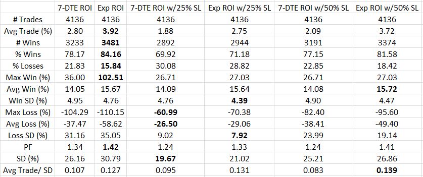
Calculated on net MR, here are the results for TF of $0.16/contract:
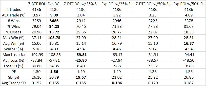
Following are the results for $0.06/contract TF based on net MR:
I generally find these numbers more encouraging than the bullish iron butterfly because the latter is not profitable with TF greater than $0.06/contract. The PCS is marginally profitable even with TF $0.26/contract. Reducing TF to $0.06 increases the average PCS trade to 3-5% profit, which is 24-40% annualized.
Unlike a butterfly, the PCS has risk in one direction only. This dramatically increases the probability of profit.
Like a butterfly, magnitude of losses are a problem with the average PCS loss being 2-4x the average win. I thought the 7-DTE exit would cut out the worst losses but it reduces profit as well. The best performing trade seems to be holding to expiration with a 50% SL although I would also seriously consider the 25% SL for risk-adjusted reasons.
Categories: Backtesting | Comments (0) | Permalink