Naked Put Backtesting Methodology (Part 4)

I continued last time talking about fixed notional risk. When backtesting this way, limited notional risk results in decreased granularity and significant error.

To better understand this, I listed the strikes used throughout the 15-year backtest in a spreadsheet. For each strike I calculated contract size corresponding to a defined notional risk. I then rounded and determined the error as a percentage of the calculated contract size. I started by keeping a cumulative tally of the error to see how that differed across a range of notional risk. Error may be positive or negative depending on whether the calculated contract size is rounded down or up, respectively. The cumulative tally therefore went up and down over the range of strikes and was not very helpful.

I then looked at the maximum and minimum values of cumulative error. This is what I found:

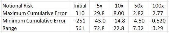
The greater the notional risk used, the lower the range of cumulative error. This illustrates the granularity issue. More granular (larger) position sizing means decreased error. Decreased error means more stability in notional risk, which I am attempting to hold constant throughout.

Backtesting my account size would have limited contract size significantly and introduced a large amount of error due to the lack of granularity. I therefore decided to increase notional risk (250x) to minimize error.

One question that remains is whether I have created an artificial situation that is incompatible with live trading. More than anything else, I am trying to get a good sense of maximum drawdown when trading this way and for this reason, I believe backtesting will provide useful information unlike any backtesting results I have seen before.

Naked Put Backtesting Methodology (Part 3)

In my last post I described the need to keep short delta as well as notional risk constant in order to have a valid backtest throughout. Today I delve deeper into implications of maintaining constant notional risk.

Notional risk can be held relatively constant by selecting proportionate contract size. Contract size is calculated by dividing the desired (constant) notional risk by the option strike price multiplied by 100. The strike price in the denominator gets multiplied by 100 because the notional risk in the numerator has already been multiplied by 100.

Understanding the impact of rounding is important with regard to this “normalization” process. The calculated number must be rounded because fractional contracts cannot be traded. I would therefore round to the nearest whole number and this introduces error. For example, if the above calculation yields 1.3235 then I would trade one contract. One is 0.3235 less than the actual number, which represents an error of (0.3235 / 1.3235) * 100% = 24.4%. I will get back to this shortly.

My next issue was deciding what notional risk to apply. Since I was going to spend several weeks on a backtest, I decided to select a value similar to my live trading account so I could get a feel for what drawdowns I might actually see.

Trading this level of notional risk resulted in a range of contract sizes from 5 to 1. The latter is problematic because as the underlying price continues to increase into the future, the one contract would represent increasing—not fixed—notional risk. No matter how high this becomes, I cannot decrease because zero contracts is no trade.

Aside from this floor effect for contract size is a problem with granularity. By multiplying the notional risk by five, I found that over the range of strikes used in my 15-year backtest, contract sizes varied from 25 to 4. This is much less granular than the 5-to-1 seen above and would result in a much smaller error.

I will illustrate this granularity concept in the next post.

Naked Put Backtesting Methodology (Part 2)

Last time I began to describe my naked put (NP) backtesting methodology. I thought I implemented constant position sizing—important for reasons described here—but such was not the case.

I held contract size constant and collected a constant premium for every trade. How could I have gone wrong?

The first thing I noticed was a gradual shift in moneyness of the options traded. I sold options with a constant premium. Earlier in the backtest this corresponded to deltas between 9-13. Later in the backtest this corresponded to deltas between 5-9. Pause for 30 seconds and determine whether you see a problem with this.

Click here

Do you have an answer?

The probability of profit is greater when selling smaller deltas than it is when selling larger ones. The equity curve would probably be smoother in the latter case with relatively large drawdowns. These are different trading strategies.

Even selling constant-delta options left the equity curve with an exponential feel, however. As discussed here, exponential curves do not result from fixed position size. I did notice the growing premiums collected during the course of the backtest but I thought by normalizing delta and contract size I had achieved a constant position size.

If you’re up to the challenge once again, take 30 seconds to figure out what’s wrong with this logic.

Figure it out?

The root of the problem is variable notional risk. Normalized delta and fixed contract size does not mean constant risk if strike price changes. Remembering the option multiplier of 100 for equities, a short 300 put has a gross notional risk of $30,000. Later in the backtesting sequence when the underlying has tripled in price, a short 900 put has a gross notional risk of $90,000. Returns are proportional to notional risk (e.g. return on investment is usually given as a percentage) and this explains the exponential equity curve.

So not only did I need to hold delta constant, I also needed to normalize notional risk. A constant contract size is not necessarily a constant position size. The latter is achieved by keeping notional risk constant and calculating contract size accordingly.

I will continue with this in the next post.

Naked Put Backtesting Methodology (Part 1)

I’ve run into a buzzsaw with regard to my naked put (NP) backtesting so I want to review the development of my methodology to date.

I started with a generalized disdain for the way so much option backtesting is done regarding fixed days to expiration (DTE). Quite often I see “start trade with X DTE.” I believe this is a handicap for two reasons. First, I can only backtest one trade per month. This limits my overall sample size. Second, I don’t believe anything is special about X DTE as opposed to X + 1, X + 4, X – 5, etc. Since they should be similar, why not do them all? This is similar to exploring the surrounding parameter space and would also solve the sample size problem.

To this end, I backtested the NP trade by starting a new position on every single trading day. This is not necessarily how I would trade in real life because I might run out of capital. However, the idea was to see how the trade fares overall. This would give me over 3500 occurrences and that is a very robust sample.

From the very beginning, my aim was to keep position size fixed to ensure drawdowns were being compared in a consistent manner. In the first backtest I therefore sold a constant contract size of naked puts with defined premium (first strike priced at $3.50 or less).

This large sample size gave me a healthy set of trade statistics. I had % wins (losses). I had average win (loss) and largest win (loss: maximum drawdown). I had average days in trade (DIT) for the winners (losers). I had standard deviation (SD) of the winners (losers) and of DIT for both. I had the profit factor. I was also able to compare these statistics to a long shares position by creating a complementary shares trade over the same time interval. I then calculated the same statistics and the NP strategy seemed clearly superior.

The analysis thus far was done to study trade efficacy rather than, as mentioned above, to represent how the trade would be experienced live. To further develop the latter guidelines I would need to generate and study an equity curve. Thankfully I already had a fixed-position-size backtest so I could at least compare the drawdowns throughout the backtesting interval.

Upon further review, however, I discovered some problems that I will describe in the next post.

Stop at the Equity Curve (20) (Part 3)

The end-of-trade PnL equity curve filter looked promising but mark-to-market (MTM) is what I would encounter in real-time.

To do this, I replicated a previous backtest from 5/1/2008 through 3/16/2009 and tracked daily account value. The 239 days between 6/17/2008 and 2/4/2009 was the shortest elapsed time to get four exit signals.

I expected the MTM equity curve to largely parallel the equity curve generated previously. I expected some evidence of future shift since the end-of-trade PnL (spreadsheet) approach counts the final trade PnL on the date of trade inception:

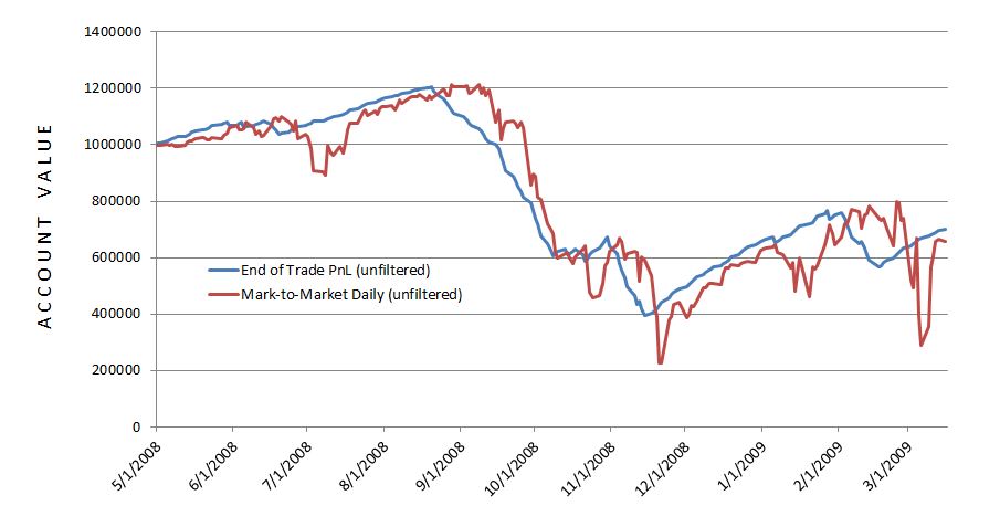
The future shift is evident along with much more volatility in the MTM daily curve. With regard to filter efficacy:

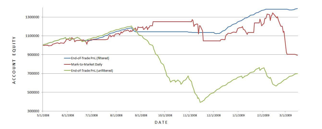
I was disappointed with MTM daily’s performance with the 20-SMA trade filter. It worked well until Feb 2009 when it suffered a very large drawdown (DD). This was the maximum DD seen with the MTM daily equity filter and a larger DD than seen without! This suggests winning (losing) days were (not) filtered out: a dangerous combination.

A closer look at the data shows the MTM daily equity filter was more active than the end-of-trade PnL filter. The former (latter) generated 13 (4) signals. Of the 13 signals, five or two lasted one or two days, respectively. This suggests a large number of whipsaws because such a filter will be effective by signalling a big market decline to remain on the sidelines for an extended period. The MTM filter was particularly ineffective in March 2009 as the strategy in the market on March 2 to lose $220K and out of the market on March 4 to miss a $175K gain.

The graph shows the MTM equity curve filter did about $200K better than no filter at all. However, with all the whipsaws I am not convinced it is any more effective. I would need a longer MTM backtest to be convinced.

Backtesting made it clear why the MTM daily filter was so much more volatile. The end-of-trade PnL method only gains or loses the value of one trade per day. Although this is big money for the largest losers, on big down days the MTM daily filter method loses big money on all of the open trades.

While the end-of-trade PnL filter was quite effective, as I suspected it is very artificial and looks nothing like the MTM daily filtered equity. If I want to continue studying an equity curve approach then I should backtest over a longer period. Alternatively, I could look to price action of the underlying for DD minimization.

Stop at the Equity Curve (20) (Part 2)

Consider this a manuscript in reverse. Having detailed the problems and limitations last time, today I will present the eye-popping, artificial results.

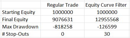
Here are the total return and drawdown numbers:

Here are the overall system statistics:

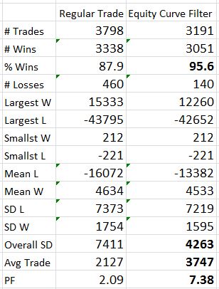
The filter clearly did a good job of removing losing trades. I highlighted the numbers that really tell the difference. The filter removed 607 trades but the % wins increased from 88% to over 95%, the overall standard deviation was reduced by 42%, and the average trade was 76% higher!

The Profit Factor went from solid to a ridiculous 7.38. This number is high enough to be worrisome. Aside from the caveats I mentioned last time, no slippage was factored into the stops so I know performance would not be this good.

The next step is to backtest several months and mark-to-market daily. I can even make sure to input the same trades as used last time. I want to see how the shape of the equity curve compares and see if significant differences exist between drawdowns.

If that ends up similar then the next step will be to study long puts. With the MA undercut 30 times, I have many instances to study in order to see how a delta-neutral position fares.

Once that’s done, I need to investigate the parameter space for MA period.

Stop at the Equity Curve (20) (Part 1)

What happens when the equity curve is used as an indicator to be in or out?

To study this, I used my -0.10/3x spreadsheet with 3,798 trades. As an arbitrary starting point, I used a 20-SMA (current day included) to be calculated after the close. When necessary, I waited one whole trading day to take action.

What’s particular about this approach is the methodology by which I have simplified the equity calculations but logistics must be considered when transitioning to real-time application. The final gain/loss registered at trade close is added to the account at trade inception. This creates the appearance of more continuity in the spreadsheet than might actually be experienced.

Consider a big down day that pushes multiple trades to maximum loss. The spreadsheet shows the total equity and MA after each trade is tabulated but in reality they would all be closed at once. This could significantly reduce the efficacy of the risk-management tool. From a mark-to-market perspective, it is conceivable that cumulative losses on many trades might drive equity below its moving average before any single trade actually closes for max loss. I’m afraid the only way to compare the two would be to backtest again and track daily equity in this manner. Hopefully it will become clear after a small sample.

When I traded naked strangles, I anecdotally noted great potential savings were I to have exited positions after incurring the greatest daily loss over the last several weeks and staying out of the market entirely until I saw a weekly equity gain. This makes me think there might be something useful about monitoring EOD equity vs. the moving average but I also wonder if this might be accompanied by more whipsaws.

Aside from timing issues, another issue requiring careful consideration is the position neutralization itself. Slippage would be horrific if I tried to close an inventory of legs especially if I had to replace them a few days later. I might be better off creating a delta-neutral position by purchasing NTM options and holding until the equity curve crosses above once again.

Having said all this, I’ll run through the results in my next post.

Musings on Put Credit Spreads (Part 8)

Today I will continue to ramble on about some possibilities of backtesting the put credit spread.

I could stick with the naked put and buy a unit or two for a fixed percentage of the naked put premium. After backtesting a put spread I was thinking about including insurance like this as a ratio backspread. Maybe what I am really talking about here are two distinct backtests—naked puts and long options—that I overlay and sum to generate an equity curve. If this is valid then I would be killing two birds with one stone because the put spreads would not have to be backtested.

Alternatively, I could opt to buy the same number of longs as I short in the back month. The extra time could synthetically substitute for the additional contract especially because for any given series of shorts, two longs would be in place. I might not include this additional bonus for backtesting purposes since each trade would consist of the naked put plus a farther out-of-the-money option in the following month. Nevertheless, I feel a sense of comfort anytime I have reason to believe actual results would be better than those backtested.

Practically speaking, a problem here is the availability of deep-out-of-the-money strikes in the database. This is especially the case in the early years (2001-4). I should call OptionVue and ask why the strikes displayed are limited and what it would take to be able to see 5-10 more strikes automatically generated by the software.

As it is now, I need to add those strikes manually and then set the prices to fit some logical vertical skew. The skew I employ is 1.0%-1.2% IV per 10 underlying points or, in subjectively perceived crash conditions, 1.5%-2.0%. Of course, too, 10 points is much larger percentage of the underlying early in the database compared to later.

After the last eight posts, I’m not sure I have solved my problem with backtesting put credit spreads. I do think everything is on the table in front of me to mull over and consider, though. I will go forth in my writing from here.

Musings on Put Credit Spreads (Part 7)

That last sentence strikes me as quite profound.

For the sake of backtesting, given these two choices I should go with the one offering a decent sample size. Discretionary traders make a [temporary?] living trading based on small sample size. Trading system salespeople use small-sample-size examples as presentation material (e.g. fallacy of the well-chosen example). I want to limit the chance of something unexpected happening, though, and a small sample size puts me at risk.

From a marketing standpoint it can’t hurt to be net long puts. I cannot reliably backtest efficacy because the number of cases where they would have saved my bacon is so few. Especially because I have to believe “my worst drawdown is always ahead,” though, long puts are insurance against something horrific. I feel confident in saying that while the broad market has never gone to zero, if people are exposed to huge risk should that happen then they would be reluctant to invest. On the flip side, while the broad market has never gone to zero, if being net long puts would result in windfall profits should that happen then people would feel quite secure about investing.

It couldn’t hurt to have both, either. Maybe I should choose a conservative profit-taking target and also buy an extra long option to serve as catastrophic insurance.

Getting back to the matter of the spread backtesting itself, my deliberation led me to believe going wider on the spread might be necessary to overcome slippage. The greater credit received would somewhat offset slippage but result in a lower ROI and it wouldn’t help in a market crash where slippage would be gigantic either way. It’s a bit sad if I have to widen the spread simply for the sake of backesting but I may have to since I don’t know how spreads have traded in real time.

I could aim for a fixed credit but that might result in variable short deltas and probability of profit. As the underlying increases in price, a fixed option premium is available farther OTM. I am assuming this would pertain to spreads too although with the long option offset, I really don’t know for certain until I look at some historic data.

Musings on Put Credit Spreads (Part 6)

3AM Eternal! My last entry was not actually posted at 03:00 and that was the April Fools joke. These days I sleep in the middle of the night unless it’s a rare weekend. Classic song, though…

In any case, I left off considering some possible ways to avoid the slippage problem.

Another possibility would be to incorporate slippage as a(n) discount (exaggeration) to profits (losses). A ballpark number I have in mind is 3%. If I sell a 10-point spread for $0.60 and close it for $0.10 then I make ~5% on it. If I discount that to 2% then I make $0.20, which is about $0.14 slippage per spread traded (leaving $1/contract for commissions).

I should expect execution to deteriorate in fast-moving markets. Since I don’t vary execution in backtesting, I should be liberal with slippage to get a realistic average. I’m not sure $0.14 per spread quite accomplishes that.

A few years ago I backtested 100-point put spreads. I intended to let the long option expire worthless, which cut slippage. The exception was when the market moved down significantly causing the long option to increase in value. With a profit-taking rule I could realize a gain before the market reverses causing the option to expire worthless. This would also prevent me from realizing a huge gain in the rare situation no reversal takes place. While a material difference exists between the two, it may be a moot point if the small sample size lacks enough consistency for future relevance.

More specifically, over the last 15 years a deep-out-of-the-money put would have gained material value roughly 11 times. These include: Sep 2001, summer 2002, June 2006, Jul 2007, Jan 2008, fall 2008, winter 2009, May 2010, summer 2011, Aug 2015, and Jan 2016. Of these 11, I’m more certain about seven (significant volatility increases). I could divide and say it happens every 16-24 months but that is an artificial construct. It happens so infrequently that I should not be surprised to go multiples of 16-24 months without experiencing it.

Inclusion of a profit-taking rule will realize more consistent profits at the cost of a few huge gainers. I cannot determine whether this is roughly equal because of the small sample size, though. This is a rare instance where 15+ years of data is probably not enough. It might amount to the difference between having a quantifiable profit-taking rule and the undefined potential of purchasing a lottery ticket.