Backtester Development (Part 10)
Posted by Mark on December 30, 2022 at 06:49 | Last modified: June 22, 2022 08:36I stumbled upon a couple further bugs in the second half of this post. Today I want to at least get started on the first one.
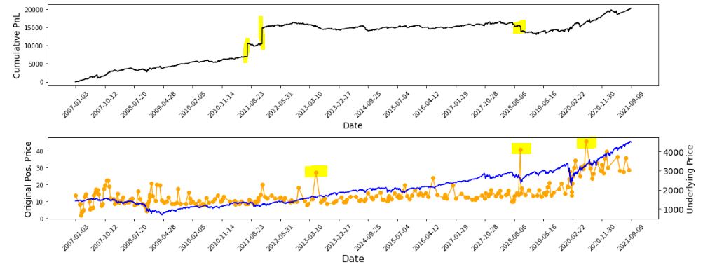
All of this started with the graph below and the highlighted point:
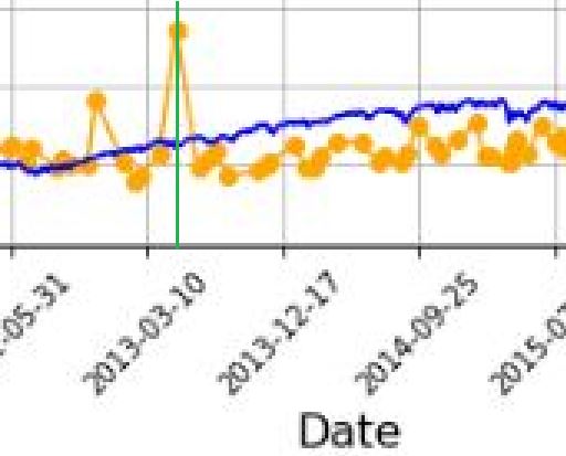
In looking to verify that [locally outlying] trade price, I expected to find early Apr 2013. In fact, the trade in question begins on Jun 21, 2013. Alarmed by the discrepancy, I suspected although the graph appears okay being packed with 255 points (trades), a closer look may reveal the points to be misaligned with dates.
Before going any further, I really should have checked to see if this is true (it is). Let’s do that right now:
I added a green, vertical line with MS Paint and calculated the distance between the green line and the previous vertical grid line (3-10-2013) as a fraction of the distance from the previous and following (12-17-2013) vertical grid lines. The fraction is 0.208, which places the date at May 5, 2013. The point is off by 47 days. That may not be much for a graph that spans over 14 years, but I thought computers didn’t make mistakes?!
It then occurred to me that while successfully getting the x-axis tick labels horizontally spaced, the points on the graph are also uniform even though the intervals between dates are not.
Once again, before going any farther I should have checked to see if this is true. Look closer at the second graph. Does the horizontal spacing look even to you? To me it doesn’t, but how can I verify?
I could do something like this:
P_price_orig_zeroes = [ 0 for i in P_price_orig_all ]
axs[1] . plot ( trade_list, P_price_orig_zeroes, marker=’o’, color=’g’ )
This creates a shadow line to the orange with equal x-values but all y-values set to zero:
Along the green line at the bottom, I have highlighted in yellow (punctuated by a few red arrows in case the highlighting is unclear) where the points are farther apart and the green line exposed.
As it turns out, the points do not align with dates but the horizontal spacing is not uniform, either. I now suspect the latter is due to the second bug I mentioned in the link from the first paragraph.
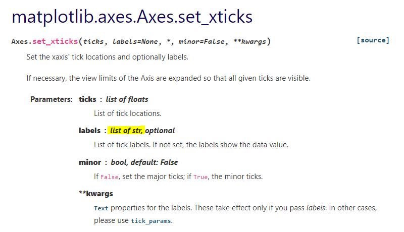
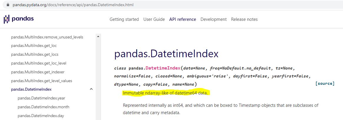
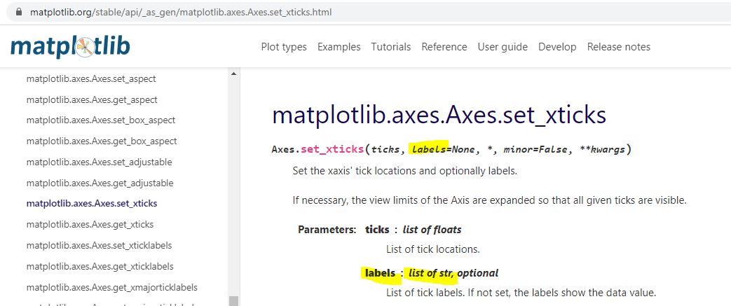
With regard to a possible cause for the irregular spacing, the code uses ax.set_xticks(). This is similar to plt.xticks() for which I included some documentation here. Looking closely at the former:
This establishes a list of strings as tick labels. Failure of the points to correctly align with label values (dates) makes sense for arbitrary strings as opposed to meaningful datetime objects. For correct alignment, maybe I can’t use ax.set_xticks() at all.
I want to correctly plot datetimes, but I want uniform tick labels rather than labels only where x-coordinates exist to match.
How can I make that happen?
Categories: Python | Comments (0) | PermalinkTime Spread Backtesting (Part 2)
Posted by Mark on December 27, 2022 at 06:25 | Last modified: June 23, 2022 14:26Last time, I began easing into time spread backtesting with my Python automated backtester by discussing trade verification. Before getting into that, I need to flush out a couple bugs in the program.
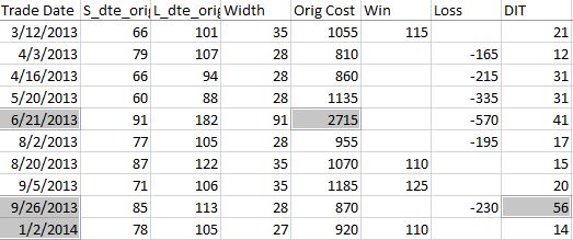
Because sudden equity jumps in the first graph may be seen as other anomalous prints on the other three graphs, I will begin with the three outlier position prices seen on the second graph. The first appears to be ~$30 around the beginning of Apr 2013. As an original price, this should be visible in the summary file:
Although the trade in question is obviously from 6/21/13 ($27.15 * 100/contract = $2,715 original cost), it plots closer to the beginning of Apr 2013. I think the problem is everything I did here with regard to “plots the evenly-spaced date labels at evenly spaced locations on the x-axis.” Unfortunately, the trades are not evenly-spaced. Although I want the tick marks to be evenly spaced in time and distance across the graph, I want the x-values of the points to correctly match the x-axis.
This will need fixing.
Another problem regards the final trade of 2013 beginning Sep 26 and lasting 56 days. Rounding off, the next trade should begin around Nov 26 (two months later). Surprisingly, the next trade does not begin until Jan 2, 2014. What happened?
I am tempted to think any open trade at the end of a year gets erroneously junked in favor of a new trade beginning first trading day of the following year due to an iteration technicality.
However, the anomaly does not seem to reduce to anything that consistent. It does not repeat for 2014 (trade ends Dec 19 with next trading starting Dec 31). It is not applicable for 2015 (Dec 22 trade correctly carries over to Jan 7, 2016) or beyond. Going backward from 2013, the anomaly does present in 2012 and in 2010.
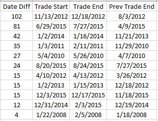
To pin this down more accurately, I replaced the Trade Date column in summary_file with Trade Start and Trade End columns. In Excel, I then subtracted the previous Trade End from Trade Start and sorted this Date Diff column from highest to lowest. Because I was missing the previous trade ending date, I inserted that as a new column making sure to Paste Special by values to prevent sorting triggering a recalculation:
Date differences of four or less are within normal limits. One would be a new trade starting on a weekday after the previous trade ended yesterday. Two could be a weekday market holiday such as Independence Day coming in between. Three would be a new trade starting on a Monday after the previous trade ended on Friday. Four would be a trade ending on a Thursday or Friday with new trade starting the following Monday or Tuesday due to a Friday or Monday market holiday.
I could even stretch to explain a five in case the market were closed for an extended period. For example, due to Hurricane Sandy the markets were closed Monday, Oct 29, and Tuesday, Oct 30, 2012.
As shown above, the list skips from four straight to 12. This defies any explanation. If the data files are clean, then I expect entries and exits on back-to-back trading days every single time.
There’s something going on…
Categories: Backtesting, Python | Comments (0) | PermalinkTime Spread Backtesting (Part 1)
Posted by Mark on December 22, 2022 at 06:39 | Last modified: June 13, 2022 14:30Bumps and bruises are still to come along the road ahead, but Version 14d of my backtester is at least somewhat functional. I am now ready to start presenting and interpreting results.
Let’s start with something very basic. In rough terms, SPX_ROD1 time spread strategy is as follows:
- If flat, then open one contract with short leg 2-3 months to expiration and long leg 4-5 weeks farther out in time.
- Exit trade if ROI% > +10% profit target or ROI% < -20% max loss.
Here are the results:
- 257 trades
- 196 winners (~76%)
- Average profit $221
- Average loss $383
- Profit factor of 1.86
In case this seems like a legit backtest, be aware of some things that are missing:
- Trade verification
- Exploration of time stops
- Exploration of alternative exit levels
- Max excursion analysis
- Drawdown analysis
- Position sizing
- Transaction fees
Looking at a summary line in isolation hides a lot of critical information. Things like cost, DIT, width, closing PnL—pretty much anything, really—should be evaluated in relation to surrounding trades to reveal potential errors. I may have coded incorrectly, or I may have a corrupt data file. I have not done my due diligence if I can’t verify by looking through a trade one day at a time to check for reasonable consistency. This isn’t to say I need to look through every trade in every backtest every time, but I should at least do some periodic spot checking.
I already have some means to do this spot-check verification. I have two output files with summary and intratrade statistics as well as four graphs [shown below in two separate screenshots] that I spent a lot of time debugging (e.g. this mini-series):
The first graph is an equity curve. Any sudden jumps are things that I want to inspect. I have highlighted three. I remember summer 2011 as a volatile market. I’m not sure about mid-2018. I will take a closer look at the trade log.
The second graph shows trade prices in orange. Any significant spikes are worthy of investigation to make sure nothing more than isolated volatility is responsible for the short-term outlier. I have highlighted three spikes on the graph.
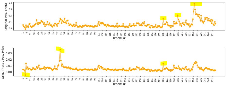
The third graph shows position theta at trade inception. I have highlighted three spikes worthy of a closer look.
The final graph normalizes initial position theta by trade cost. I have highlighted three spikes that are worthy of investigation. The first of these is clearly below zero, which suggests either theta or cost starts out negative. I can hardly imagine either one of those given accurate data so I definitely want to analyze that.
I will continue next time.
Categories: Backtesting, Python | Comments (0) | PermalinkBacktester Development (Part 9)
Posted by Mark on December 19, 2022 at 06:29 | Last modified: June 22, 2022 08:37Today I want to finish updating what I have for backtester logic beginning with other considerations regarding maximum excursion (ME; see end of Part 8).
I’m not convinced that I need to report ME in btstats. As the statistic itself refers to an intratrade value, I can only think of two reasons to include it in the intraday report: to see how it changes over the course of the trade, which doesn’t matter to me, or to see exactly when it occurs, which I know anyway because I store that number separately ( _dte). All the context I probably need is in summary_results where I will also see initial DTE and DIT.
Besides, comparing ME across trades is easy in summary_results but much more difficult in btstats. In the former, each row corresponds to one trade and looking at ME across trades is as simple as scanning from row to row. In the latter, multiple rows correspond to each trade and I would need to do a lot of scrolling and looking up ‘WINNER’ or ‘LOSER’ in trade_status.
Removing ME from btstats will simplify an if-elif-else to if-else since ‘WINNER’ and ‘LOSER’ are otherwise handled the same.
And if trade_status is ‘WINNER’ or ‘LOSER,’ then before continuing data file iteration the program proceeds to:
- Assign ‘INCEPTION’ to trade_status
- Assign ‘find_spread’ to control_flag
- Reset all variables (fifth-to-last paragraph of Part 7 aside)
- Assign True to wait_until_next_day
I added a profit factor calculation to summary_results by:
- Appending two more rows (dictionaries) for mean and count of wins and losses by doing
summary_results = summary_results.append ( { } ) [not just summary_results.append()] - Calculating PF_calc by using .iloc[ ] to look up particular values
- Appending a row at the bottom to display PF_calc
Finally, I once again had to debug the graphing portion having to do with the x-axis tick labels that I discussed here, here, here, and here. I end up resolving this with three lines:
L1: xtick_labels = pd.date_range (btstats [‘Date’] . iloc[0], btstats [‘Date’] . iloc[-1] , 20 )
This creates a list of 20 evenly-spaced trading dates including the first and last.
L2: xtick_labels_converted = xtick_labels . strftime ( ‘%Y-%m-%d’ )
This is needed to avoid ConversionError [“Failed to convert value(s) to axis units”] from L3.
L3: axs[0] . set_xticks (list (np . linspace (1, len (btstats . index), num = \
len (xtick_labels_converted) ) ), xtick_labels_converted, rotation = 45)
This plots the evenly-spaced date labels at evenly spaced locations on the x-axis.
Technically speaking—and these are the details on which I get hung up and confused as a beginner—pd.date_range() in L1 returns a Datetimeindex. How do we know that and what does it mean?
I can do an internet search for pd.date_range:
I can do an internet search for datetime index:
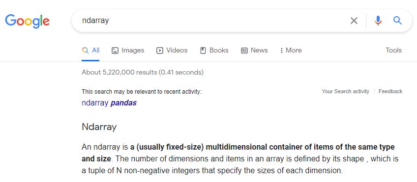
Is “ndarray-like” bad English? An internet search turns up a page that explains this, too.
Ndarray can also be better understood by an internet search:
I don’t know much about arrays yet, but I do know they are a different data type from what [an internet search has informed me that] ax.set_xticks() is expecting:
Type str[ing] rather than [type] array or Index is expected. The Datetimeindex has large integers that nobody would want to see as tick labels anyway. L2 converts those to strings with a familiar character format (YYYY-MM-DD).
That pretty much covers the updated logic for this version of the backtester.
Categories: Python | Comments (0) | PermalinkGPN Stock Study (2-13-23)
Posted by Mark on December 16, 2022 at 07:05 | Last modified: March 8, 2023 14:08I recently* did a stock study on Global Payments Inc. (GPN) with a closing price of $117.88.
CFRA writes:
> Global Payments (GPN) provides payment processing and software
> solutions globally through a variety of distribution channels,
> which enable customers to accept card, electronic, check, and
> digital-based payments. Specific offerings include
> authorization, settlement, funding, customer support,
> chargeback, security, and billing services.
This medium-sized company has grown sales and earnings at annualized rates of 14.5% and 6.5% over the last 10 years, respectively. Visual inspection is not great. Revenue data is [missing for ’16 and] down in ’18 while EPS data is [missing for ’16 and] down in ’15, ’18, ’19, and ’20. Q2 and Q3 2022 EPS have declined sharply. [Stock] Price bars in ’17 and ’22 overlap, which represents several years without significant appreciation. PTPM, which averaged 14.6% from ’12-’14, has averaged 11.5% over the last five years. Although apparently in decline, this beats peer and industry averages.
ROE has averaged 4% over the last five years, which seems low. The industry averages 6%, though, while peers average 6.8% (both excluding ’20, which is -161% or worse). Debt-to-Capital, which ranged from 51.1% (’12) to 75.5% (’14) between ’12-’18, has averaged 28% over the last three years. The latter is less than peer and industry averages. Quick Ratio and Interest Coverage are a concerning 0.53 and 1.4, respectively.
The fact that so many analysts are covering this company gives me some [hopefully not illusory] assurance about its liquidity. Aside from all the analysts represented below, M* says the balance sheet is sound. Value Line gives a B++ financial strength grade and says “it should continue to easily meet its various obligations.” CFRA says expected FCF generation ($2.2B and $2.5B in ’22 and ’23, respectively) should allow leverage to return to historical levels by the end of ’23.
I assume long-term annualized sales growth of 8% based on the following:
- CNN Business projects 4.9% YOY growth and 6.6% per year for ’22 and ’21-’23, respectively (based on 27 analysts).
- YF projects YOY 6.3% and 9.2% growth for ’23 and ’24, respectively (24 analysts).
- Zacks projects YOY growth of 6.6% and 2.6% for ’23 and ’24, respectively (7).
- Value Line projects annualized growth of 8.3% from ’21-’26.
- CFRA projects 3.9% YOY contraction for ’23.
- M* provides a 2-year ACE of 1.6% growth and 8% growth per year through ’26 (analyst note).
I assume long-term annualized EPS growth of 10% based on the following:
- CNN Business projects 10.4% YOY and 12.5% per year for ’22 and ’21-’23, respectively (based on 27 analysts), along with 5-year annualized growth of 14.8%.
- MarketWatch projects 12.5% and 11.5% per year for ’22-’24 and ’22-’25, respectively (31 analysts).
- Nasdaq.com projects 11.8% YOY growth for ’24 (10 and 2 analysts for ’23 and ’24).
- Seeking Alpha projects 4-year annualized growth of 17%.
- YF projects YOY 11.4% and 14.5% for ’23 and ’24, respectively (24), along with 5-year annualized growth of 15.1%.
- Zacks projects YOY 9.9% and 13.6% for ’23 and ’24, respectively (7), along with 5-year annualized growth of 15.8%.
- Value Line projects annualized growth of 13.7% from ’21-’26.
- CFRA projects 14.5% YOY for ’23 and 3-year projected annualized growth of 15%.
- M* provides a long-term estimate of 16.6%.
My forecast is below the range of six long-term estimates (mean 15.5%).
As Q2 and Q3 of ’22 were atypically soft ($0.13 and $0.17/share, respectively), I will not originate the earnings projection from there. Given trendline ($2.90) or ’21 ($3.29), I choose the former (more conservative).
My Forecast High P/E is 35. Over the last 10 years, high P/E has trended up from 18.6 (’12) to 67.1 (’21) excluding upside outliers of 85.8 and 110.6 in ’19 and ’20. The last-5-year average (excluding outliers) is 49.2.
My Forecast Low P/E is 28. Over the last 10 years, low P/E has trended up from 14.3 (’12) to 35.5 (’21). ’19 and ’20 were high at 45.6 and 54.1, but not to an extreme. The last-5-year average is 38.3.
My Low Stock Price Forecast is $92.10. In projecting from the trendline, I also need to manually override EPS (to $2.90) rather than defaulting to TTM ($0.17) for calculation of the Low Stock Price Forecast. This is 21.9% below previous close, equal to the 52-week low, and below both ’20 and ’21 low stock prices.
Payout Ratio was below 3% in ’18 and earlier before averaging 25.8% over the last three years. I will assume 10% to be conservative.
All this computes to an U/D ratio of 2.6, which makes GPN a HOLD. The Total Annualized Return is 9.8%, but PAR (using Forecast Average, not High, P/E) is 7.5%: less than I want out of a medium-sized company.
To better interpret this, I use Member Sentiment (MS) to assess the study’s margin of safety (MOS). Out of 50 studies over the past 90 days (my own and two others with invalid low prices excluded), projected sales, projected EPS, Forecast High P/E, Forecast Low P/E, and Payout Ratio average 9.3%, 22.2%, 44.4, 29, and 13.9%, respectively. My inputs are all lower. Value Line projects an average annual P/E of 40, which is higher than MS (36.7) and me (31.5). MOS seems robust here.
MS has an extreme Low Stock Price Forecast of $63.83. This is over 30% lower than mine and below the 2017 low price. Eleven studies are in the single digits, which leaves me scratching my head. From the lowest price in the last three months to now, GPN has rallied 26.5%. This may explain some of the forecasts, but not those under $30/share.
Excluding these 15 studies, I get an MS Low Stock Price Forecast of $87.42, which seems more reasonable. This would equate to a Forecast Low P/E of 26.5 in my study. I will stick with my $92.10 because my forecast P/E range is low enough already.
*—Publishing in arrears as I’ve been doing one daily stock study while posting only two blogs per week.
Backtester Development (Part 8)
Posted by Mark on December 13, 2022 at 07:02 | Last modified: June 22, 2022 08:37Today I will continue (see end of Part 7) with backtester logic for maximum excursion (ME).
I will begin talking about the output files. Two dataframes are created with pd.DataFrame(): btstats for intratrade monitoring and summary_results for end-of-trade reporting. These are ultimately converted to .csv files with pd.to_csv().
Rows are added sequentially to the dataframes upon completion. For btstats, add_btstats is created where each list element corresponds to a dataframe column. Minimal calculation in this list statement (e.g. L_iv_orig x 100) could have been done with variable assignment if I renamed the variables to reflect it. Index of the last record is then used to add list to the bottom:
> btstats.loc [ len ( btstats . index ) ] = add_btstats
In contrast to adding rows as lists, I build summary_results by adding rows as one dictionary per trade:
> summary_results = summary_results . append ( { ‘Trade Num’ : len (trade_list) }, ignore_index = True)
This is a long line with a key-value pair for every column (only one of which is shown here). The final argument is needed when appending a dictionary to avoid a TypeError.
Pandas documentation says DataFrame.append() has been deprecated in favor of .concat(). I do not get any such warning. A closer look suggests the deprecation pertains to adding one dataframe to another. I am adding a dictionary.
Now that I have described the structures in which ME will be reported, let’s talk about ME itself. By definition, MFE (favorable) is the farthest a trade goes in my favor before ending up a loser and MAE (adverse) is the farthest a trade goes against me before ending up a winner. Strictly speaking, a losing (winning) trade has no MAE (MFE).
However, a useful application might involve running trades from start to finish without profit targets or max losses to record largest intratrade loss and gain. Plotting the two against each other can then give an idea whether a particular stop level might lock in more winners to the exclusion of losers or avoid locking in more losers to the exclusion of winners. All this is contingent on knowing whether intratrade gain or loss comes first. I have the _dte variables to tell me that.
To allow for such application, I define MFE (MAE) to be maximum intratrade gain (loss) without regard to trade outcome. My tweak is to recognize MFE (MAE) for winning (losing) trades as the previous day’s MFE (MAE) before stop level is hit.
Needing to differentially apply current or previous ME when stop levels are checked after ME is updated makes the program logic more complicated. For trade_status ‘IN_TRADE,’ I report MAE and MFE. For ‘WINNER’ (‘LOSER’), I report MAE and MFE_prev (MAE_prev and MFE). All this leaves me with three different add_btstats lines that need to be properly fit into an if-elif-else block. The same goes for summary_results.
I will continue next time.
Categories: Python | Comments (0) | PermalinkTGT Stock Study (2-12-23)
Posted by Mark on December 8, 2022 at 06:43 | Last modified: March 8, 2023 10:36I recently* did a stock study on Target Corp. (TGT) with a closing price of $170.02.
Value Line writes:
> Target Corp.’s operations consisted of 1,926 discount stores,
> of which 1,528 were owned, in the U.S., mostly in Cal., Tex.,
> and Fla (as of 1/29/22)… Sales by category in fiscal ’21:
> beauty/household, 26%; hardlines, 18%; apparel/accessories,
> 17%; food, 20%; and home furnish., 19%.
This mega-sized company (annual revenue > $50B) has grown sales and earnings 3.4% and 13.1% per year over the last 10 years, respectively. Lines are mostly up except for dips in sales (’16) and EPS (’13 and ’16). PTPM over the last decade has ranged from 4.3% (’14) to 8.4% (’21) with a last-5-year average of 5.9%. This is higher than peer and industry averages.
ROE has trended up over the last 10 years from 18% (’12) to 32.5% in ’20 (’21 was an upside outlier at 48.1%) with a last 5-year average (excluding ’21) of 28.1%. This is higher than peer and industry averages. Debt-to-Capital has increased from 49.4% (’12) to 56.2% (’21) with a last-5-year average of 53.1%. This is also higher than peer and industry averages. Current Ratio is a suboptimal 0.86, but Interest Coverage is 10.8. M* assigns an Exemplary capital allocation rating while Value Line gives a B++ grade for financial strength.
I assume long-term annualized sales growth of 2% based on the following:
- CNN Business projects 2.5% YOY and 2.2% per year for ’22 and ’21-’23, respectively (based on 31 analysts).
- YF projects YOY 2.3% and 2.2% for ’23 and ’24, respectively (29 analysts).
- Zacks projects YOY 2.3% and 2.8% for ’23 and ’24, respectively (12).
- Value Line projects 3.8% annualized growth from ’21-’26 (11% from ’20-’26).
- CFRA projects growth of 2.8% YOY and 2.3% per year for ’23 and ’22-’24, respectively.
- M* provides a 2-year ACE of 2.1% and a 10-year estimate of 3% in its analyst note.
My estimate is just below all of the above.
I assume long-term annualized EPS growth of 2% based on the following:
- CNN Business projects a 59.3% YOY contraction and 17% contraction per year for ’22 and ’21-’23, respectively (based on 31 analysts), along with 5-year annualized contraction of 4.2%.
- MarketWatch projects annualized contraction of 15.9% and 5.5% for ’22-’24 and ’22-’25, respectively (36 analysts).
- Nasdaq.com projects annualized growth of 42.6% and 36.5% for ’23-’25 and ’23-’26, respectively [16, 10, and 2 analysts for ’23, ’25, and ’26].
- Seeking Alpha projects 5-year annualized growth of 10.5%.
- YF projects 59.1% YOY contraction and 70% YOY growth for ’23 and ’24, respectively (33), along with 5-year annualized contraction of 4.9%.
- Zacks projects 59.2% YOY contraction and 71.4% YOY growth for ’23 and ’24, respectively (16), along with 5-year annualized growth of 9.9%.
- Value Line projects annualized growth of 5.8% from ’21-’26.
- CFRA projects 56.8% YOY contraction and 15.9% contraction per year for ’23 and ’22-’24, respectively, and 1% growth per year from ’21-‘24%.
- M* projects long-term annualized growth of 4.8%.
I am projecting below the average [of six] long-term estimate[s] (3.6%).
I will override to project earnings from the last annual data point rather than Q3 ’22. Analyst consensus expects a big rebound in earnings for ’23, which is suggestive of a one-year anomaly due to the macroeconomic factors rather than maturation in business cycle. The latter has already occurred for this company.
The ideal situation would be to project from the same point analysts are using for their calculations, but because this is not explicitly disclosed, I have to do my best to work around it. Here, projection from the last quarterly data point or EPS trendline makes no sense because Forecast High Stock Price would be at or below the current stock price.
My Forecast High P/E is 17. Over the last 10 years, high P/E has ranged from 14.6 (’12) to 23.9 (’13) with a last-5-year average of 18.8.
My Forecast Low P/E is 10. Over the last 10 years low P/E has ranged from 9.1 (’17) to 18.2 (’13). The last-5-year average is 10.6. As suggested above, I think Target is a mature company so I don’t expect the kind of P/E compression that might be seen with a younger, more explosive growth company.
I’ve realized that I need to be very careful with the website and future EPS projection. Overriding the base on the estimated EPS growth rate screen leaves TTM EPS for the Low Stock Price Forecast. The latter may require changing as well.
My Low Stock Price Forecast is $137. The default value would be $141. This corresponds to ’21 earnings of $14.10/share and assumes 0% growth for the next five years. With the 52-week low price at $137.2, I’m overriding with $13.70/share to [roughly] match. $137 is 19.4% below the previous close.
Over the last 10 years, Payout Ratio has ranged from 22.4% (’21) to 51.5% (’13). The last-5-year average is 37.2%. I am assuming 31%.
All this computes to an U/D ratio of 2.9, which makes TGT a HOLD. The Total Annualized Return is 11.1%, and PAR (using Forecast Average, not High, P/E) is 6.6%, which is less than desired. Can I convince myself that the inherent margin of safety (MOS) in this study allows for a good chance of realizing Forecast High P/E?
To answer this, I compare my inputs with the larger sample size of Member Sentiment (MS). Out of 192 studies over the past 90 days (my own and four others with projected low prices above last closing price excluded), projected sales, projected EPS, Forecast High P/E, Forecast Low P/E, and Payout Ratio average 4.7%, 7.8%, 18.4, 11.3, and 38.4%, respectively. My inputs—especially the growth rates—are all lower. Value Line projects an average annual P/E of 15, which is barely higher than MS (14.9) and higher than mine (13.5). All this is indicative of a healthy MOS.
MS provides a[n] [average] Low Stock Price Forecast of $97.58, which is 28.8% lower than mine. It’s also closer to the 2020 [COVID crash] low of $90.20. In my opinion, a stock price five years from now > 20% below today’s price is almost unfathomable for [even] a[n] [anemic] growth company. This legitimizes my Low Stock Price Forecast. Forecasting close to the ’20 lows almost seems preposterous. I’d be curious to know if these MS studies were accompanied by a manual EPS override.
A significantly lower Low Stock Price Forecast would move TGT further into the Hold zone, but because this seems unreasonable I choose to ignore it as an offset to the MOS. The only remaining question in my mind is why CNN Business (FactSet) and YF (Refinitiv) project negative 5-year earnings growth when the other four do not.
That concern aside, I feel comfortable with TGT as a BUY under $169/share.
*—Publishing in arrears as I’ve been doing one daily stock study while posting only two blogs per week.
Backtester Development (Part 7)
Posted by Mark on December 5, 2022 at 07:16 | Last modified: June 22, 2022 08:37Today I will finish discussing the ‘find_spread’ control branch before moving on to ‘update_long.’
A few final steps are taken after the spread is identified:
- All variables are assigned from lists.
- First row of btstats (intratrade_results) is added.
- trade_status is changed to IN_TRADE.
- Control flag gets assigned ‘update_long.’
- Several variables and lists are reset. This includes converted_date.
- Break out of the for loop.
The last step is critical. I initially included a continue statement, which repeats the loop and selects the longest-dated option under 200 DTE every time: definitely not what I want.
I’m somewhat confused in determining where the program goes next, but I think it must be back to the top of the data file iteration loop. The for loop, of which this is a part, concludes the ELSE of the ‘find_spread’ control branch. Unlike the previous version, at this point the program is already looking at the next date so nothing needs to be done with wait_until_next_day.
The ‘update_long’ branch is brief. If strike price and long expiration date match, then variables for the long option are updated along with underlying price. If strike price and expiration date do not match, then continue to the next line of the data file.
I am sloppy with what variables to reset at the end of ‘find_spread.’ Some variables not reset are used in ‘update_long.’ What matters most is that every variable to be subsequently passed to btstats gets assigned a new value as part of the update branches. I’ve discussed possibly using functions to initialize and reset variables. Much of the resetting (and initializing) is unnecessary as long as I assign everything at the proper points. I try and reset where I can since I don’t trust myself with this, but I could shorten the program simply by being more careful.
The ELSE, which executes when control_flag is ‘update_short,’ begins with a check to make sure current_date still matches historical date. False would indicate the spread failed to be updated: a fatal flaw.
Next and similar to above, if strike price and short expiration date match, then variables for the short option and the spread are updated. No need to change underlying price as date has not changed.
I then include logic for max adverse/favorable excursion. I need variables for MFE, MAE, MFE_dte, and MAE_dte. I also need to store the previous values because I never want the max excursion to be equal to closing PnL.* If ROI_current < MAE (or > MFE), then the MAE (MFE) values get assigned to a _prev variable set and ROI_current gets assigned to MAE (MFE).
I will continue next time.
*—Alternatively, I could have used and maintained lists with two elements
each rather than duplicating the variable set with a _prev suffix.
ULTA Stock Study (2-11-23)
Posted by Mark on December 1, 2022 at 07:23 | Last modified: July 18, 2023 13:49I recently* did a stock study on Ulta Beauty, Inc. (ULTA) with a closing price of $515.75.
M* writes:
> With roughly 1,350 stores and a partnership with narrow-moat
> Target, Ulta Beauty is the largest specialized beauty retailer
> in the U.S. The firm offers makeup (43% of 2021 sales),
> fragrances, skin care, and hair care products (20% of 2021
> sales), and bath and body items. Ulta offers private-label
> products and merchandise from more than 500 vendors. It also
> offers salon services, including hair, makeup, skin, and brow
> services, in all stores. Most Ulta stores are approximately
> 10,000 square feet and are in suburban strip centers.
This medium-sized company has grown sales and earnings at annualized rates of 15.7% and 16.6% over the last 10 years, respectively. The stock price has hardly seen a reprieve. Lines are mostly up, straight, and parallel except for an EPS decline in ’20. PTPM over the last decade has increased from 12.6% to 15% with a last-5-year average (excluding ’20, which was a downside outlier) of 13.3%. This is higher than BBWI (a peer) and industry averages.
ROE has increased from 24.2% to 47.3% over the last 10 years with a last-5-year average (excluding ’20) of 38.5%. This outpaces BBWI and industry averages. Debt-to-Capital was 0% until 2019 and has averaged 51.3% over the last three years (lower than BBWI and industry averages). This is all uncapitalized leases as the company has zero long-term debt.
I assume long-term annualized sales growth of 7% based on the following:
- CNN Business projects 16.3% YOY and 11.5% per year for ’22 and ’21-’23, respectively (based on 24 analysts).
- YF projects YOY 15.7% and 7.3% for ’23 and ’24, respectively (28 analysts).
- Zacks projects YOY 15.8% and 7.8% for ’23 and ’24, respectively (10).
- Value Line projects 4.4% annualized growth from ’21-’26 (12.5% from ’20-’26).
- CFRA projects growth of 15.6% YOY and 10.1% per year for ’23 and ’22-’24, respectively.
- M* provides a 2-year ACE of 12.1% and a 10-year estimate of 7.5% (analyst note).
I assume long-term annualized EPS growth of 8% based on the following:
- CNN Business projects 28.2% YOY and 16.3% per year for ’22 and ’21-’23, respectively (based on 24 analysts), along with a 5-year annualized growth of 12.7%.
- MarketWatch projects annualized growth of 18.9% and 14.8% for ’22-’24 and ’22-’25, respectively (29 analysts).
- Nasdaq.com projects 7.2% and 7.9% growth per year for ’23-’25 and ’23-’26, respectively [14, 8, and 1 analyst(s)].
- Seeking Alpha projects 4-year annualized growth of 23.9%.
- YF projects YOY 27.3% and 5.6% for ’23 and ’24, respectively (30), along with 5-year annualized growth of 12%.
- Zacks projects 5.6% YOY for ’24 and a 5-year annualized growth of 13.8% (14).
- Value Line projects 8.9% annualized from ’21-’26.
- CFRA projects 26.1% YOY and 12.8% per year for ’23 and ’22-’24, respectively, along with 23% per year from ’21-’24.
- M* provides a long-term estimate of 11%.
I am projecting well below the average [of seven] long-term estimate[s] (15%).
My Forecast High P/E is 23. Over the last 10 years, high P/E has ranged from 20 (’21) to 42.1 (’13) excluding the upside outlier in ’20 (99.8). The last-5-year average is 29.6 (excluding ’20). This has been trending lower.
My Forecast Low P/E is 15. Excluding the upside outlier in ’20 (39.9), over the last 10 years low P/E has trended down from 28.4 to 15.8. The last-5-year average (excluding ’20) is 18.1.
My Low Stock Price Forecast is the default value of $341.30. The 52-week low price is $330.80, which makes this reasonable despite being 33.8% below the last closing price. The stock has been on a tear lately.
All this computes to an U/D ratio of 0.9, which makes ULTA a HOLD. The Total Annualized Return is 5.3%, and PAR (using Forecast Average, not High, P/E) is 2.6%: less than the current yield on T-Bills.
To assess margin of safety (MOS) in this study, I compare my inputs with Member Sentiment (MS). Out of 536 studies over the past 90 days (my own and eight others with projected low prices above last closing price excluded), projected sales growth, projected EPS growth, Forecast High P/E, and Forecast Low P/E average 10.7%, 10.7%, 29.5, and 20.8, respectively. My inputs are all lower. Value Line projects an average P/E of 22, which is lower than MS (25.1) and higher than mine (19).
MS has a Forecast Low Stock Price of $287.67, which is ~15% below mine. This is no surprise given that the stock has rallied ~20% over the last three months; for many studies, this was calculated when the stock was lower.
Despite a decent MOS, I await prices under $423/share to revisit ULTA.
*—Publishing in arrears as I’ve been doing one daily stock study while posting only two blogs per week.

