Put Credit Spread Study 1 (Part 3)
Posted by Mark on September 29, 2017 at 06:34 | Last modified: August 1, 2017 09:05Last time I presented initial results for the put credit spread (PCS) backtest. Rarely does a trade actually average TF of $0.26/contract, though, so today I will look at smaller values.
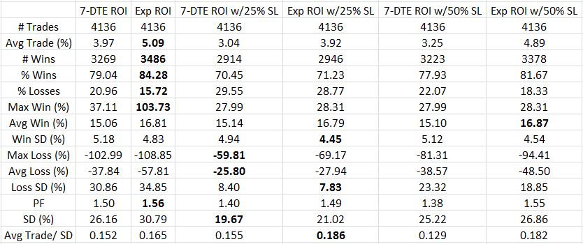
Calculated on net MR, here are the results for TF of $0.16/contract:
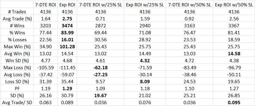
Following are the results for $0.06/contract TF based on net MR:
I generally find these numbers more encouraging than the bullish iron butterfly because the latter is not profitable with TF greater than $0.06/contract. The PCS is marginally profitable even with TF $0.26/contract. Reducing TF to $0.06 increases the average PCS trade to 3-5% profit, which is 24-40% annualized.
Unlike a butterfly, the PCS has risk in one direction only. This dramatically increases the probability of profit.
Like a butterfly, magnitude of losses are a problem with the average PCS loss being 2-4x the average win. I thought the 7-DTE exit would cut out the worst losses but it reduces profit as well. The best performing trade seems to be holding to expiration with a 50% SL although I would also seriously consider the 25% SL for risk-adjusted reasons.
Categories: Backtesting | Comments (0) | PermalinkPut Credit Spread Study 1 (Part 2)
Posted by Mark on September 26, 2017 at 05:42 | Last modified: August 1, 2017 08:53Today I will start presenting results for my first put credit spread study.
The global disclaimer is to say no winner really exists in the “best performing trade” competition. What is most meaningful to me may be less meaningful to you. This is why alignment between a trade strategy and individual personality is so important. All I can do is explain my interpretation of these numbers. You will have to do the same.
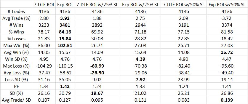
Here are the results for TF = $0.26 using net MR (see last post for explanation of table contents):
The first thing I look at is PF followed by risk-adjusted return. Exp barely edges out Exp w/50% SL for PF and vice versa for Avg Trade/SD. I would therefore trade Exp w/50% SL because this gives me a better chance of avoiding the biggest losses. Looking at the SD data gives me pause because I really like seeing drawdowns minimized. Perhaps a better comparison to put this in proper context would be to compare against $4,000 of long shares daily (as done in the last link).
Given the choice between exiting trades at 7 DTE or Exp, the latter seems to outperform. Avg Trade, PF, and Avg Trade/SD all reflect this in the comparisons between rows 2 vs. 3, 4 vs. 5, and 6 vs. 7.
Two things are missing from this rationale, though, with the first being max loss. 7 DTE has smaller max losses than Exp each time. That makes sense with the rapid option decay of the final week. Max loss can significantly limit position size. In thinking about strategies with max loss -100% vs. -50%, I would trade the former much smaller. Do remember, though, that in trading like I backtest my position size would be relatively small simply in virtue of putting a new trade on every single day. This not only gives me a large sample size but it also dilutes drawdowns.
Especially in thinking about this “perpetual scaling” approach, the risk-adjusted return is more important to me than max loss. As mentioned, expiration outperforms 7 DTE every time.
The second missing piece from the performance comparison is trade duration. The expiration trade is seven days longer. Annualized ROI would be one way of factoring this in because the same average trade would have a lower ROI per year if held to expiration than 7 DTE. PnL per day would be even more direct.
Next time I will study the impact of TFs.
Categories: Backtesting | Comments (0) | PermalinkPut Credit Spread Study 1 (Part 1)
Posted by Mark on September 21, 2017 at 04:58 | Last modified: August 1, 2017 08:51After less than two months (personal record!) I now have initial data to present for put credit spreads.
The arbitrary parameters are as follows:
–Sell first strike < 0.30 delta (less fudge factor for OV inconsistency)
–40-point spread width
–Exit at 7 DTE or 1 DTE
–Stop-loss (SL) levels -25% or -50% based on net margin
–Transaction fee (TF): $0.26/contract
This is a daily backtest using 3:30 PM ET data from 1/2/2001 – 6/21/2017 (4,136 trades). When the OV database was incomplete I went to 3:00 PM or 4:00 PM and/or filled in with theoretical values.
Margin requirements (MR) for credit spreads may be presented as gross or net. Net MR subtracts initial credit received from spread width multiplied by 100. This makes for larger winners and losers on a percentage (ROI) basis compared to gross MR and therefore increases standard deviation. I evaluated trades based on net MR.
Remembering my previous discussion about TFs, I recalculated results for $0.16/contract and $0.06/contract. One further consideration is that some losers near SL cutoffs might become winners (e.g. decreasing TF by $0.10 equates to an improvement of 1% in ROI on gross margin). I did not include the flips in the performance calculations.
Results of the backtest will be presented in forthcoming tables with bold type reflecting the best values (most positive for winners and least negative for losers) for each performance metric (row). Average Trade is mean ROI across all trades. SD is standard deviation. PF is profit factor. SD in the penultimate row of each table is calculated across all trades. The last row (Avg Trade/SD) is a risk-adjusted return.
The performance metrics were calculated for six (columns) exit combinations. 7-DTE ROI reflects trades closed with seven days to expiration. Exp ROI includes trades closed on expiration Thursday (1 DTE). 7-DTE ROI w/25% SL tabulates the first value of MAE to exceed 25% or ROI at 7 DTE if the threshold is never breached. Exp ROI w/25% SL uses Exp ROI if that 25% threshold is never breached. 7-DTE ROI w/50% SL tabulates the first value of MAE to exceed 50% or ROI at 7 DTE if the threshold is never breached. Exp ROI w/50% SL uses Exp ROI if that 50% threshold is never breached.
I will present the tables next time.
Categories: Backtesting | Comments (1) | PermalinkQuestioning Butterflies
Posted by Mark on September 18, 2017 at 06:26 | Last modified: June 10, 2017 07:31I feel like I could go on with BIBF discussion for quite some time but I think it may be time to change course altogether.
In the final paragraph of my last post, I laid out a solid plan for future research directions. I now have five degrees of freedom, which are multiplicative in trading system development. This could easily take years of manual backtesting.
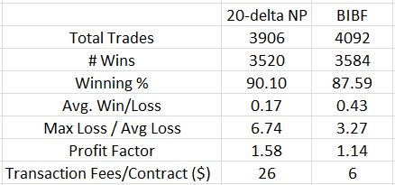
I find it hard to accept this significant time commitment given the disappointing first impression for butterflies when compared to naked puts (NP). Consider NPs versus the BIBF:
These numbers somewhat confirm my NP worries about the potential for large downside loss. Max Loss / Avg Loss is 2.1x greater for the BIBF. Average win/loss metric is 2.52x greater for the BIBF. In both cases, advantage: butterflies.
But to get the BIBF looking this good, I had to significantly reduce transaction fees. I question whether I can reliably get these trades executed for so little slippage on each side. If not then up to 319 of the 4092 backtested trades [with MAE = 0] are at risk of going unfilled, which means the backtested performance is artificially high.
The BIBF performance is hardly compelling. A profit factor of 1.14 is just slightly into the profitable range. 1.58, for the NPs, is much more to my liking especially being saddled with a healthy amount of transaction fees at $26/contract. Whereas 1.14 may be optimistic, 1.58 may be pessimistic.
One other thing to notice is the much larger commission cost for butterflies over NPs. Trading NPs is dirt cheap: one or two commissions per position. Trading butterflies involves at least six commissions per position and possibly 7-8. All that and I get less profit? This is a soft poke in the eye.
If the real challenge is to limit potential for catastrophic downside risk then perhaps the better way to proceed is with put spreads or put diagonals.
Another idea is to consider a bearish butterfly as a hedge for trading NPs since the latter will be hurt by a down market whereas the former could benefit. I’d be interested to see how a bearish butterfly performs compared to this bullish one but I would be inclined to implement fixed width, which would mean two additional lengthy backtests.
Categories: System Development | Comments (0) | PermalinkBullish Iron Butterflies (Part 8)
Posted by Mark on September 14, 2017 at 07:01 | Last modified: June 8, 2017 14:07Trading system development is, for me, a learning process and backtesting butterflies has been no different. This post is good background. What I found out last time was a real problem with the concept of width-adjusted MAE.
To be more specific, I do not believe width-adjusted MAE allows for an apples-to-apples comparison across trades. I came up with the “width-adjusted” concept here to correct for the fact that narrow [breakeven] trades seem to hit max loss more often. With regard to MAE, which is related to stop-loss, normalizing for width means the narrowest trades are most diluted in terms of ROI. That is to say the narrower the trade, the more unlikely it is to be stopped out.
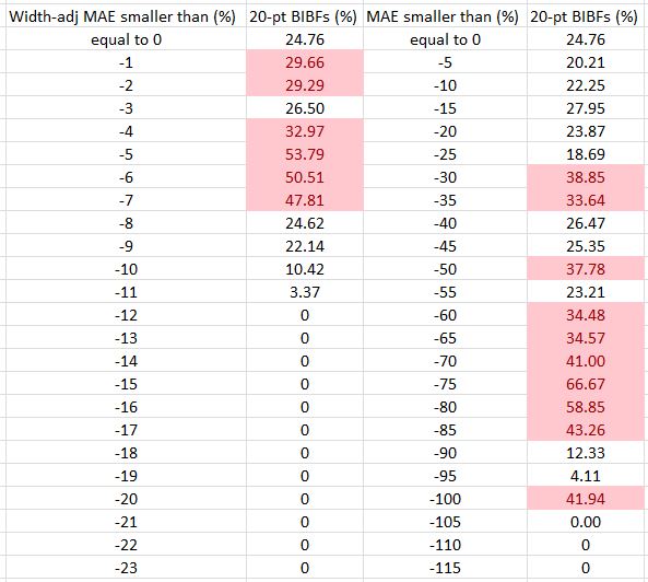
To quantify this, I will study the percentage of 20-point BIBFs across both width-adjusted and non-adjusted MAE categories. I previously calculated that 28.6% of all trades were 20-point spreads. In the following table, cells colored red include a proportion of 20-point BIBFs that exceeds 28.6%:
Indeed, narrow butterflies are more prevalent in the higher percentages of the non-adjusted MAE distribution while being more prevalent in the lower percentages of the width-adjusted MAE distribution. A stop-loss triggering on width-adjusted PnL would therefore be less likely to stop out narrow BIBFs than if based on non-adjusted PnL. Unfortunately the narrow BIBFs are most in need of a stop-loss.
Part of me thinks this is an absolute mess.
Another part of me thinks this is just a reflection of the level of complexity I’m dealing with here.
From a backtesting perspective, this might be an argument for using constant spread width regardless of underlying price. That would eliminate the need to normalize for width altogether. The question would then be what width to use. Perhaps backtesting 20-, 40-, 60-, and 80-point wide spreads would be sufficient for comparison.
Selecting a constant spread width would once again introduce a new degree of freedom into the equation. This variable would be in addition to exit day (introduced in last post), stop-loss (not yet identified), profit target (arbitrarily selected as 10%), and short strike selection (arbitrarily selected as 2-3% above the money).
Categories: Backtesting | Comments (1) | PermalinkBullish Iron Butterflies (Part 7)
Posted by Mark on September 13, 2017 at 06:20 | Last modified: June 7, 2017 13:31In need of a cure for these beautiful, sunny late-spring mornings? How about looking at maximum adverse excursion (MAE) distributions! Today I will proceed using the approach I described at the end of my last post.
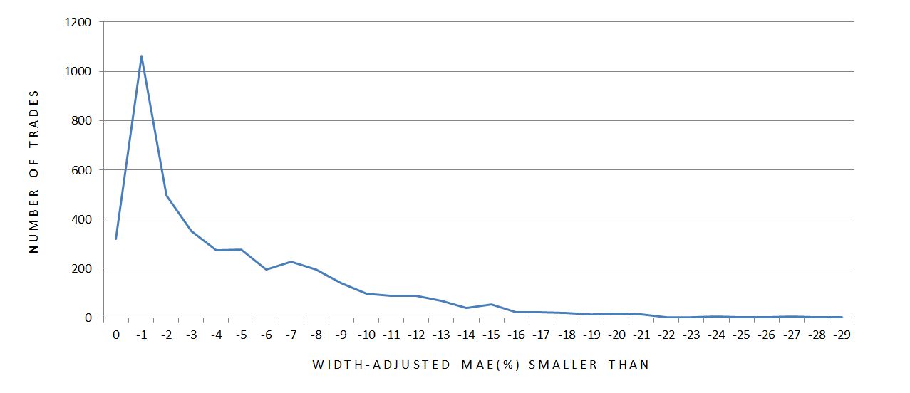
What follows is a histogram of width-adjusted MAE. Total number of trades is plotted for every integer along the x-axis. Zero corresponds to the number of trades with width-adjusted MAE of zero. -1 on the x-axis corresponds to trades with width-adjusted MAE between 0 and -1%, -2 on the x-axis corresponds to trades with width-adjusted MAE smaller than -2% down to -1%, -15 corresponds to trades with width-adjusted MAE smaller than -15% down to -14%, etc.
Some of the cumulative percentage numbers are worth noting here. 7.80% of all trades have zero MAE. 54.4% of all trades have MAE smaller than -3%. 88.8% and 99.2% of all trades have MAEs smaller than -10% and -20%, respectively.
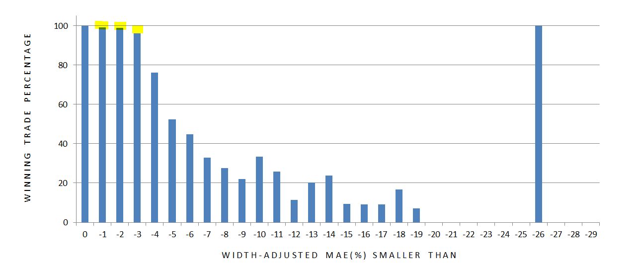
The percentage of winning trades in each group can help determine whether MAE distribution may be effectively used to define a stop-loss. A clear argument for a stop-loss threshold would be a PnL value having all winning trades on one side and all losing trades on the other:
What surprised me was the presence of losing trades having such small MAEs (see yellow highlighting). Out of the 319 trades with zero MAE, 319 trades won: no surprise there. Out of the 1062, 495, and 351 trades with MAE smaller than -1%, -2%, and -3%, however, I had eight, six, and 14 losers, respectively. To be down so little during the lifetime of the trade yet not end up hitting the profit target is extremely unusual with the time-decay acceleration taking place into expiration.
A big market move on expiration Thursday could help to explain this. MAE includes PnL numbers from trade inception through 2 DTE while “expiration PnL” is tracked in another column. One reason I backtested this way was to identify big moves occurring late. I have strong suspicion of such a move wherever I have a maximum favorable excursion (MFE) occurring with < 7 DTE followed by a losing trade at expiration.
All of this is important because large losing trades in the face of small MAEs diminish the potential benefit of a stop-loss. One way to prevent this might be to exit all trades at 7 DTE and avoid expiration week altogether. This introduces “exit day” as another degree of freedom, though, which puts me at greater risk for the curse of dimensionality.
Before studying MFE and a date distribution for the losing trades described above, I see a bigger problem potentially lurking that should be addressed first.
I will talk about this next time.
Categories: Backtesting | Comments (0) | PermalinkBullish Iron Butterflies (Part 6)
Posted by Mark on September 8, 2017 at 06:07 | Last modified: June 2, 2017 14:55So far I have done several things with the BIBF analysis: considered the impact of transaction fees (TF), looked at width-adjusted ROI, identified a relationship between spread width and underlying price, and looked at performance stratified by implied volatility. Today I want to talk about maximum adverse excursion (MAE).
I have two issues to address before looking at MAE distribution: TF and width normalization. I like to remain as plain vanilla as possible in my analysis to minimize chances of curve-fitting. This means not implementing one condition then overlaying another on top of that then a third on top of the first two, etc. Adhering to the “plain vanilla” guideline could mean leaving the $26/contract TF and not normalizing for spread width.
I would be more willing to conduct the analysis this way if it didn’t differentially affect trades. At $26/contract, the total TF is $208/trade. Given $735 as the average cost for a 20-point butterfly, starting down $208 means the minimum MAE is -28.2% (and -52% for the cheapest trade of $400!). The wider butterflies are affected less due to the larger denominator.
Aside from this TF-induced-apples-to-oranges MAE comparison, the whole concept of being in loss at trade inception seems questionable. Yes, slippage is a reality of trading and this is a logical way of accounting for it. Intuitively, though, I feel MAE should be zero when the trade is placed.
Reducing TF to $6/contract would cost me $48/trade, which is a 77% reduction. For the average 20-point butterfly this is -6.5% (-12% for the cheapest 20-point butterfly). This feels small enough to be tolerable while still acknowledging the reality of slippage. Unfortunately this still affects narrow butterflies more than wider ones. In the true spirit of MAE, I think I must normalize for TF by adding back the $208 for each trade.
The discussion is similar with regard to spread width. Narrow-butterfly PnL seems to be skewed toward the loss side while normalizing for spread width mitigates this effect. To some degree this is a position sizing issue (how many contracts per $10,000?), which I would prefer to leave out of the system development process altogether. Because of the large effect, though, I think I have no choice but to normalize.
Next time I will study the distribution of width-adjusted MAE without transaction fees.
Categories: Backtesting | Comments (2) | PermalinkBullish Iron Butterflies (Part 5)
Posted by Mark on September 5, 2017 at 06:45 | Last modified: June 1, 2017 14:07Today I want to focus on implied volatility (IV) to better understand whether high IV offers any edge to trading the BIBF.
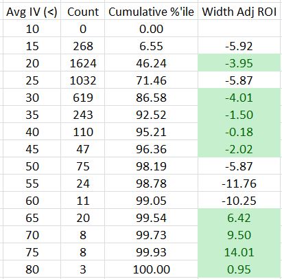
I sorted the spreadsheet by Avg IV and tabulated counts and trade results:
As expected, high IV does not occur very often: 71.46% of all trades occurred with IV under 25.
Higher IV does not seem to offer much of an edge. You may recall that the average width adjusted ROI across all trades is -4.22%. The green cells correspond to ROI numbers that are better than this and they appear scattered across IV categories.
The four exceptions are the profitable trades placed with Avg IV between 60-85.
Two things give me pause about drawing meaningful conclusions from these highest of IV levels. First, IV of 60 or greater encompasses only 0.95% of the total trades. Second, all these trades occurred between October 6 and December 12, 2008, which is a mere sliver of the 16+ years covered by the entire backtest. This short time interval also corresponds to just one market condition: the worst crash we have seen this century. I would not generalize based on such a limited sample size.
This illustrates one of the dangers of doing spreadsheet research. I put in formulas and whipped up these numbers but I still need to look over the computations and scrutinize whether they make practical sense. In this case, they appear meaningful even though they may be due solely to chance.
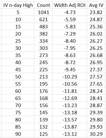
Besides comparing trades in different IV groupings, another approach is to take trades only when Avg IV equals an n-day high. This is similar to the metric of IV Rank, which is frequently discussed in trading circles. Here is the breakdown of trade performance when Avg IV hits an n (ranging from 5 to 90)-day high:
No groups show profitable average trades. I thought longer-term highs would correspond to higher IV levels, which would be more susceptible to mean-reversion thereby benefiting the BIBF. This may be happening along with big market moves at highest IV that offset the IV contraction (I have seen this before). I can tell that longer-term highs are selecting conditions with higher IV (including the most volatile IV spikes, which are probably included for most values of n) because IV is directly proportional to n.
To see such a strong inverse relationship between average trade and n, though, is quick shocking to this investigator.
Just in case you’re wondering why I’m bothering to analyze these data at all with them clearly amounting to a losing strategy, I remind you that the $26/contract transaction fee is having a significant negative effect on the results.
Categories: Backtesting | Comments (0) | Permalink